Welcome
Welcome and congratulations on joining the HPC team. This is the HPC Training Book which contains the training material which will be used to train you in many of the preliminary HPC concepts required to participate in the HPC branch and in MDN as a whole. Throughout this book you will learn the basics of the C programming language, parallel and distributed computing and job batching. You will complete challenges across the weeks to test your knowledge and give you the opportunity to practice your skills.
What is HPC?
HPC stands for high performance computing. In involves using extremely powerful machines to perform complex tasks. It combines aspects of network management, parallel computing techniques and distributed computers to solve highly complex problems. The main focus of HPC is to build and use computer clusters; collections or grids of powerful computers that can communicate information between each other, to solve advanced computational problems that involve a lot of data or process power and time.
HPC at Monash DeepNeuron
The HPC branch at Monash DeepNeuron works on many different projects. Everything from creating mini clusters, to using supercomputer clusters to simulate complex, real world systems for research and technology development in may different scientific disciplines. Within the HPC branch you will learn a lot about HPC development starting with the foundational concepts and ideas involved in HPC to working on various projects that implement and utilise these techniques in order to solve many different complex problems.
HPC Training
What is all this and what is it for?
This is a book. More specifically it is the book containing all the content, training resources and learning materials that you will be using to complete you HPC training. The purpose of this book is to provide clear and concise learning resources that you can utilise effectively; not just in your HPC training, but for the entirety of your time at Monash DeepNeuron.
What are you going to learn?
During your HPC training, you are going to learn all about HPC concepts and various tools that exist that allow us to perform HPC development. You will start with the setup process which involves downloading some tools you will be using throughout your training as well as creating a GitHub account. You will then learn about the C programming language and to effectively use it to create powerful and fast computer programs. You will then gain access to M3; Monash's cluster environment, where you will learn hwo to distribute jobs across one or many different computers. You'll also learn about concepts involved in parallel and distributed computing and development programs using these techniques to improve the speed of software applications.
Along the way you will learn how to effectively use developer tools like Git and GitHub as well as solving various challenges each week to test and practice what you have learnt in each chapter.
How to use this book
Using the book is pretty self explanatory. The content is split up into chapters which covers a particular topic which can be further broken down sections. You navigate through the book mostly chronologically using the arrow buttons on either side of the page (can't miss them). You can also look through the chapters and sections to find particular topics or using the search bar, which can be activated by pressing S. Each chapter has a challenges section. These contain various tasks to complete related to the content of each chapter.
Contributing
You can contribute to the book by accessing its GitHub repository (GitHub log in the top right hand corner of any page). Follow the contributing guidelines on the repository for more details.

Getting Started
In this chapter you'll setup some essential software tools that you will be using throughout your training. Note that some sections are specific to particular platform and devices. Only complete the section that is specific to your platform. The GitHub section you must complete no matter which platform you are on.
GitHub
Git. What is it?
Git is a Source Control Management tool (SCM). It keeps a history of multiple files and directories in a bundle called a repository. Git tracks changes using save points called commits. Commits use .diff files to track the difference in files between commits. Repositories can have multiple branches allow many different developers to create new changes and fixes to a codebase that are separate from each other. You can also switch between branches to work on many different changes at once. These branches can then later be merged back together to a main branch, integrating the various changes.
What is GitHub?
GitHub is a remote Git service. This allows you to store Git repositories online so that individuals and teams can access and work on Git repositories and projects remotely. It offers many features on top of basic version control such as branch, issue and feature tracking, releases, CI/CD pipelines, project management and more. Its predominately used through its website which offers control of these features through a simple GUI. Throughout your time at Monash DeepNeuron, university and probably for the rest of your career (if in a software based role), you will use service like GitHub to help management the development of projects.
Your first task is to sign up for a GitHub account, if you haven't already. I would highly recommend using a personal email address (not a university one) as you will most likely want access to your account after university.
It is also a good idea to install the GitHub mobile app. This allows you track and manage projects and reply to messages and issues from your phone.
Joining Monash DeepNeuron's GitHub Organisation
Once you have signed up for GitHub, you will need to provide your instructors with your GitHub username. This is so we can invite you as a member of the Monash DeepNeuron's organisation on GitHub. This will give you access to projects and allow you to communicate with other members. This will also allow you to gain specific privileges for your future projects at Monash DeepNeuron. You're invitation to the organisation will be sent via the email used for your account.
Watching Repositories
GitHub allows you 'watch' repositories. This means you'll be notified of changes to the repository so that you can keep on top of is happening with various projects. You'll be using this later in your training.
Download GitHub Mobile
We would also request you install the GitHub mobile app. This can make it easier to login to your account (2FA), interact in discussions, reply to mentions and manage repositories and projects when you aren't at your computer.
Windows Setup
For your training you will need a few tools. Namely:
- Git
- C compiler toolchain (MSVC)
- A text editor (VSCode)
Installing Git
First, you will need to install Git. This allows you to use Git from the terminal and also gives you access to a bash shell environment. While following the install wizard, make sure to select the option that adds Git to your PATH. This important as it allows you to use Git in 'PowerShell'. Keep the other default operations. Git may require you to restart you machine.
Connect GitHub
Once Git has installed, open a new 'Git Bash' that was installed. This can be found in the Windows 'Start' menu. Once it is open, run the following commands, replacing the username and email section with your details (keeping the quotation marks).
git config --global user.name "<github-username>"
git config --global user.email "<github-email>"
Installing MSVC
Next we will need to install a C compiler toolchain. There a many different environments such as CygWin, MinGW but the most ideal environment is Microsoft's official development environment, MSVC. Download the Community Edition of Visual Studio and launch the installer. Under the 'Workloads' tab of the installer select the 'C++ Build Tools' bundle and click install. This may take a while. Once installed (may require restart) open the 'Start' menu and navigate to the 'Visual Studio' folder. There should a variety of different terminal environment applications. This is because Windows has slightly different toolchains and environments for x86 (32-bit) and x86_64 (64-bit). Select the 'Developer Command Prompt for VS 2022' app. In the terminal that spawns, run the command.
cl
This will display the help options for cl, Window's C compiler.
VSCode Installation and Setup
Now that MingW and GCC are installed and setup we will want to setup a text editor so we can easily edit and build our programs. For your training, I recommend using VSCode as it allows you to customize you developer environment to your needs. If you prefer another editor such as Neovim, feel free to use them as you please.
First download VSCode for Windows VSCode Download
Once installed, open the app and navigate to the extensions tab (icon on the left size made of four boxes). Using the search bar, install the following extensions.
- C/C++
- GitLens
- Git Graph
- GitHub Pull Requests and Issues
- Sonarlint
And thats it, you are all setup.
Mac Setup
For your training you will need a few tools. Namely:
- Xcode
- Git
- C compiler toolchain (GCC)
- A text editor (VSCode)
Installing Xcode, Git & GCC
First, we will need Xcode command line tool utilities, to do so, open the 'Terminal' app and run the following command:
xcode-select --install
This will prompt you to accept the install and will download Git and GCC onto your device. To verify installation was successful, run:
$ xcode-select -p

# Should print this
/Library/Developer/CommandLineTools
Note:
Here,
$indicates the prompt of the terminal. Do not include it in the command. This may be a different symbol on your device.
VSCode Installation and Setup
Now that Homebrew, Xcode and GCC are installed and setup we will want to setup a text editor so we can easily edit and build our programs. For your training, I recommend using VSCode as it allows you to customize you developer environment to your needs. If you prefer another editor such as Neovim, feel free to use them as you please.
First download VSCode for Mac VSCode Download
Once installed, open the app and navigate to the extensions tab (icon on the left size made of four boxes). Using the search bar, install the following extensions.
- C/C++
- GitLens
- Git Graph
- GitHub Pull Requests and Issues
- Sonarlint
And thats it, you are all setup.
Linux Setup
For your training you will need a few tools. Namely:
- Git
- C compiler toolchain (GCC)
- A text editor (VSCode)
For this section I will be assuming a Debian system, namely Ubuntu. Replace apt commands with your distributions relevant package manager.
Installing Packages
To begin, you will need to install some packages. This will be done using apt, Ubuntu's system package manager. Run the commands in the shell.
# `sudo` represents 'super user do'.

# This runs a command with admin. privileges.
# Update apt's local package index.
sudo apt update

# The `-y` flag means upgrade yes to all.
# This bypasses confirming package upgrades.
# Upgrade packages with new versions
sudo apt upgrade -y

# Installs specified packages (separated by spaces).
sudo apt install git curl wget build-essential
And that's it. Linux is setup and installed.
Connect Git & GitHub
Next we will link your GitHub account to you local Git install. Run the following commands, replacing the username and email section with your details (keeping the quotation marks).
git config --global user.name "<github-username>"
git config --global user.email "<github-email>"
VSCode Installation and Setup
Now that GCC is installed and setup we will want to setup a text editor so we can easily edit and build our programs. For your training, I recommend using VSCode as it allows you to customize you developer environment to your needs. If you prefer another editor such as Vim, Emacs or Neovim, feel free to use them as you please.
First download VSCode for Linux VSCode Download
Once installed, open the app and navigate to the extensions tab (icon on the left size made of four boxes). Using the search bar, install the following extensions.
- C/C++
- GitLens
- Git Graph
- GitHub Pull Requests and Issues
- Sonarlint
And thats it, you are all setup.
WSL Setup
For your training you will need a few tools. Namely:
- Windows Terminal
- Windows Subsystem for Linux
- Installing Ubuntu
- Git
- C compiler toolchain (GCC)
- A text editor (VSCode)
This section will cover how to install WSL on Windows. If you already have a WSL setup you can skip these steps.
Installing Windows Terminal
The first thing you will need is the new Windows Terminal app. This makes it easier to have multiple shells open, even different shells. This will be used to access your WSL instance.
Note:
Shells are an environments that allow access to the operating system (OS), hardware and other system processes through simple shell commands, usually a shell language like Bash or Powershell.
Installing and Setting Up WSL
Before you begin make sure to update Windows to make sure you have the latest version. You will then need to check in order to see if you can install WSL is if virtualization is enabled for your device. You can check this by opening 'Task Manager', clicking on the performance tab and looking at the CPU details. There will be an option called 'Virtualization' which should say 'Enabled'.
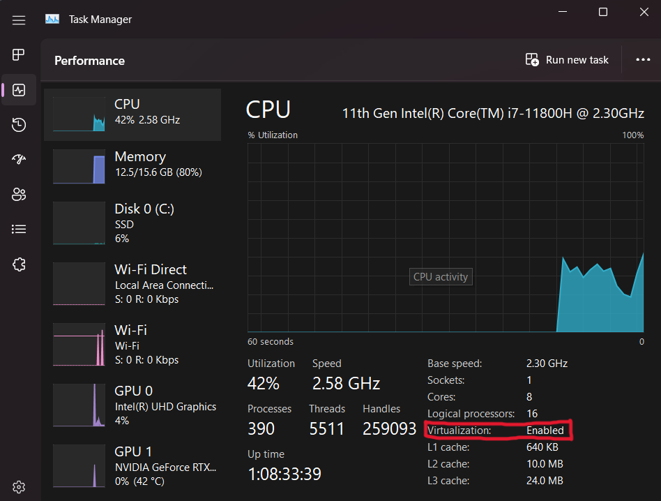
Next, open Powershell with Administrative Privileges and run the following command.
wsl --install -d Ubuntu-22.04
Once this has finished, you may need to restart your machine. With that WSL is installed. You should be able to open a Ubuntu shell using Windows Terminal by clicking the arrow icon next to the default tab and selecting Ubuntu. On your first launch, this may require you to setup your user credentials.
Installing Packages
To begin, you will need to install some packages. This will be done using apt, Ubuntu's system package manager. Run the commands in the shell.
# `sudo` represents 'super user do'.

# This runs a command with admin. privileges.
# Update apt's local package index.
sudo apt update

# The `-y` flag means upgrade yes to all.
# This bypasses confirming package upgrades.
# Upgrade packages with new versions
sudo apt upgrade -y

# Installs specified packages (separated by spaces).
sudo apt install git curl wget ca-certificates build-essential
And that's it. WSL is setup and installed.
Connect Git & GitHub
Next we will link your GitHub account to you local Git install. Run the following commands, replacing the username and email section with your details (keeping the quotation marks).
git config --global user.name "<github-username>"
git config --global user.email "<github-email>"
VSCode Installation and Setup
Now that WSL, Ubuntu and Git are installed and setup we will want to setup a text editor so we can easily edit and build our programs. For usage with WSL ans your training in general I recommend using VSCode as it allows you to customize you developer environment to your needs. It also can access the WSL filesystem allowing you to work on projects in a native Linux environment on Windows. If you prefer another editor such as Vim, Emacs or Neovim, feel free to use them as you please.
First download VSCode for Windows VSCode Download
Once installed, open the app (on the Windows side) and navigate to the extensions tab (icon on the left size made of four boxes). Using the search bar, install the following extensions.
- C/C++
- GitLens
- Git Graph
- GitHub Pull Requests and Issues
- Sonarlint
- Remote development
- WSL
- Remote SSH
You can then navigate to the window with the Ubuntu shell from before and run:
code .
This will installed VSCode on the WSL from your Windows version and open it in the home directory. And thats it, you are all setup.
M3 MASSIVE
MASSIVE (Multi-modal Australian ScienceS Imaging and Visualisation Environment) is a HPC supercomputing cluster that you will have access to as an MDN member. In this page we will set you up with access before you learn how to use it in Chapter 5. Feel free to go through the docs to learn about the hardware config of M3 (3rd version of MASSIVE) and it's institutional governance.
Request an account
In order to access M3, you will need to request an account. To do this, follow this link: HPC ID. This should take you to a page this this:

Type in Monash, as you can see here. Select Monash University, and tick the Remember my organisation box down the bottom. Once you continue to your organisation, it will take you to the Monash Uni SSO login page. You will need to login with your Monash credentials.
You should now see something like this:
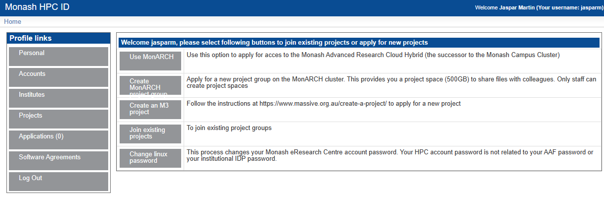
Once you are here, there are a couple things you will need to do. The first, and most important is to set your HPC password. This is the password you will use to login to M3. To do this, go to home, then click on Change Linux Password. This will take you through the steps of setting your password.
Once you have done this, you can move on to requesting access to the MDN project and getting access to gurobi.
Add to project
To request to join the MDN project, again from the Home page click on Join Exiting Project. You should see a screen like this:
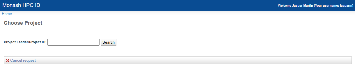
In the text box type vf38 and click search. This is the project code for MDN. Then select the project and click submit. You will now have to wait for the project admins to approve your request. Once they have done this, you will be able to access the project. This should not take longer than a few days, and you will get an email telling you when you have access.
Once you have access to everything, you are ready to get started with M3. Good job!!
Git SSH setup
In order to reliably clone git repos in M3, in particular private ones, it is best practice to use SSH cloning. This is a bit more complicated to set up, but once it is done, it is much more streamlined. There are few steps involved. First, you will need to generate an SSH key on M3. Login to M3, and run the following command:
ssh-keygen -t ed25519 -C "your_email@example.com"
This will then prompt you to enter a file location. Just press enter to use the default location. It will then ask you to enter a passphrase. This is optional, but recommended.
Once you have generated your key, you need to add it to the ssh agent. Do this by running:
eval "$(ssh-agent -s)"
ssh-add ~/.ssh/id_ed25519
You will then need to copy the public key to your clipboard. You can do this by running:
cat ~/.ssh/id_ed25519.pub
Then, go to your github account, go to settings, and click on the SSH and GPG keys tab. Click on New SSH key, and paste the key into the box. Give it a name, and click Add SSH key.
You should now be able to clone repos using SSH. To do this, go to the repo you want to clone, but instead of copying the HTTP link, copy the SSH link, and then its regular git cloning.
Nectar Cloud
The ARDC Nectar Research Cloud (Nectar) is Australia’s national research cloud, specifically designed for research computing. Like with M3, we will set you up with access now before you learn about it in later chapters. This webpage explains what it is if you're curious.
Connect Monash Account to Nectar Cloud
To create an identity (account) in Nectar Cloud, all you have to do is login using your Monash student account. Click this link to access Nectar's landing page.
You will see the following. Make sure to click "Login via AAF (Australia)".

You will be redirected to enter your Monash credentials after which you will see the Nectar Cloud dashboard for your trial project (your project name will be pt-xxxxx).
Cloud Starter Series
ARDC has provided this cloud starter tutorial series for people new to Nectar Cloud. You should be able to follow these tutorials using your trial project. If you need more SUs (service units aka. cloud credits) in order to provision more cloud resources for MDN-related work, you should message your HPC Lead with that request.
Challenges
As you progress through each chapter you will be given a small set of challenges to complete. In order to complete the challenges there is a complementary GitHub template repository found on the Monash DeepNeuron GitHub organisation called HPC Training Challenges. As a template you are able to create your own copy of the repository and complete the challenges completely independent of the other recruits.
Setting Up Challenges Repository
To get setup:
- Click the link above to go to the repository on GitHub.
- Click 'Use this template' button (green) and select 'Create a new repository'.
- Give it a name and make sure it is private.
- Ensure you are copying it to your personal account and not the Monash DeepNeuron organisation. There will be a dropdown next to where you give the repo a name from which you can select your account.
- Click 'Create repository from template'.
- This will open the page for the repository. Click the '<> Code' button (green), make sure you are in the HTTPS tab and copy the link.
- Open a terminal in your dev directory.
- Run:
# Clone to your machine
git clone <repo-link>

# Enter clone's directory
cd <repo-name>

# Create link to template called 'upstream'
git remote add upstream https://github.com/MonashDeepNeuron/HPC-Training-Challenges.git

# Disable pushing to template
git remote set-url --push upstream DISABLE

# Sync with 'upstream'
git fetch upstream

# Merge 'upstream' main branch with your main
git merge upstream/main --allow-unrelated-histories

# Open repository in VSCode
code .
This will clone the repository into you current working directory maintaining its link to its origin (your remote copy on GitHub) allowing you to sync changes between you local and remote copies. This also sets up a link called upstream to the original template directory with pushing disabled. This allows you to sync the base of the repository with your copy, similar to a fork but prevents changes from being pushed to the template.
Once you completed a challenge or made some changes you want to save to your remote repository you can simply add to a commit stage, combine the changes in a commit and then push the commit to origin.
git add .               # Add any untracked or modified files
git commit -m "msg"     # Commit changes locally with a message
git push origin         # Push to your GitHub repository
If you need to sync your local repository with the remote version you can either fetch the changes to add them to the logs without modifying the codebase or pull them to integrate the changes into your version.
git fetch origin    # Sync changes with remote without integrating (downloading) them
git pull origin     # Sync and integrate remote changes locally
In order to sync your copy of the challenges repository with the remote template you must re-fetch the changes from upstream and then merge the upstream remote with your local repository.
git merge upstream/main --allow-unrelated-histories
Note: Look at the README.md of the repo for the for more instructions.
Challenges Repository
The challenges repository is broken down into different directories for each chapter. For each chapter their will be a series of additional directories corresponding to the specific challenge. These will contain any and all the resources needed for the challenge except programs that you are required to complete.
When you want to attempt a challenge it is good practice to create a branch. This allows you to make changes to the codebase that do not affect other branches each with their own history. You can then later merge branches to integrate changes together. To create a new branch you can use the git-branch command or the the -b flag with the git-checkout command giving both the name of the new branch. This will branch from your current position in the repositories history. Switching branches is achieved using the git-checkout command (with no -b flag). You use the regular git-add, git-commit and git-push commands interact and save the changes that only affect this new branch.
git branch <branch-name>        # Create new branch
git checkout <branch-name>      # Checkout to the new branch
# or
git checkout -b <branch-name>   # Checkout to a new branch
For your training. I would recommend creating a new branch for every challenge you attempt and merging them with the main (default) branch once you are done. This allows you to make modifications to each of your attempts independent of each other as well as make it easier to resync with the template repository should anything change at its base. it also allows you to get some meaningful practice with Git which is one of the most used developer tools in the world.
When you want to merge your changes, checkout back to the main branch and run a merge request. This will pull the changes from the deviating branch into main and update it accordingly.
# On your deviant branch
git fetch origin
git checkout main
git fetch origin
git merge <branch-name>
Note: Merging sometimes creates merge conflicts. This happens when the two branches histories cannot automatically merge. Git has many tools to assist resolving these conflicts and there is a plethora of resources online to assist you. If you get stuck do not hesitate to reach out.
Brief Introduction to C
What is C?
What is C? You may have heard of a something called C in your classes or online but may be unaware of what it is and what it is used for. Simply put C is a general purpose programming language developed at Bell Labs in 1972 by Dennis Ritchie. It was designed to closely reflect the architecture and capabilities of the target device. It was popularized in large part due to its usage and role in the UNIX operating system. Before languages like C, developers and engineers had to mostly use assembly languages; the instruction code that was specific to every single device (CPU in particular), meaning an application for one device would have to be rewritten in the new devices assembly language. C aimed to make this easier, creating a unified language that could then be compiled to any target architecture. The 'write once, compile everywhere' philosophy. This dramatically increased the capabilities of developers to create portable applications that were also easier to write.
Design
C is a very simple programming language. It has relatively minimal syntax, a small standard library and only a few primitive data types and entities. C's power comes from its simplicity, it allows developers to utilise any and all components of a computer in any way the developer sees fit. This is because C is still able to target various system-level operations such as allocate memory and make system calls. This capability is derive from C originating as the language that was used to create the UNIX operating system, the predecessor of Linux and MacOS. C and UNIX were developed simultaneously meaning any operation they needed UNIX to perform had to be accessible from C. C also has a very simple memory model that closely reflects how computer memory is designed today which follows Alan Turing's original description of a Turing machine ie. memory is an infinitely (not truly infinite, but for arguments sake) long tape of individually addressable cells.
Technical Description
C is a static and weakly typed language. What are types? Types are in essence a form of structure, typically dictated by their layout ie. their size in memory. Every language has type system which dictates the operations that can be performed on a particular types and the semantics for when these operations can occur. A statically typed language means that the compiler must know the type of every piece of data in a program. This is because data has a fixed width in C meaning any program written in C must have a known size such that the it can actually run on a machine. Weakly typed describes a language for which data types are allowed to have implicit conversions. This means that you can utilise the same data but in a different shape. This is sometimes useful but more often is a pitfall to the language.
Family History
While many people will talk about the C family of languages, many of the execution techniques used in C were inspired by another language called ALGOL developed in the late 50's. Many of the principles in ALGOL were using in C. See is also the successor to the B programming language (also developed at Bell Labs by Ken Thompson and Dennis Ritchie). C has inspired almost every procedural language used today and has had a massive influence on other language families. Some of the descendants of the C language include C++, Swift, JavaScript, PHP, Rust, HolyC, Java, Go, C#, Perl and (depending who you ask) Python.
Entire (mostly) Programming Language Lineage

- Source rigaux.org
Simplified Programming Language Lineage
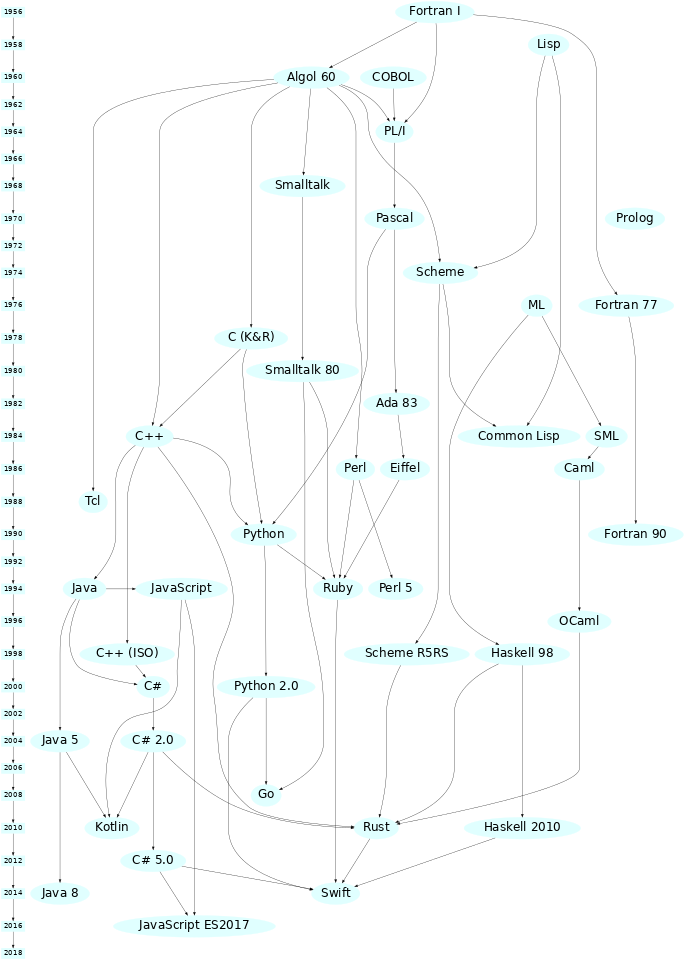
- Source rigaux.org
Hello World
If you have ever programmed before you may be familiar with 'Hello World'. If not, a 'Hello World' program is often the first program you write in a programming language. It serves a brief introduction to the languages syntax, a simple workflow in that language and also as a sanity check to ensure the developer tools for the project were installed and setup correctly.
Fun Fact:
The 'Hello World' test program was popularized by Brian Kernighan's Programming in C: A Tutorial.
Setup
To begin open a new terminal window. If you don't already have a development directory it is a good idea to create one. This should be where you host all your projects.
# Optional
mkdir dev
cd dev
In this directory (or another of your choosing) we are going to create a directory for our 'Hello World' project. Finally, we'll open VSCode in this location so that we can easily edit our code.
mkdir hello
cd hello
code .
Note:
Windows users will have to use the Developer Command Prompt used in the Windows section of the last chapter. You will then need to navigate to a different directory. Ideally use your 'Home' directory.
cd C:\Users\<username>You should be able to follow the instructions above normally.
Compiling and Running
'Hello World' in C is quite simple, although not as simple as say Python. First create a new file called main.c.
#include <stdio.h>

int main()
{
    puts("Hello World\n");
    return 0;
}
To compile and run the program simply run the commands below. The output will be an executable called main (main.exe on Windows) located in the same directory as the source file.
Linux, MacOS & WSL
gcc -o main main.c
./main
Hello World
Windows
cl main.c
main.exe

# ...

Hello World
What's Going On Here?
Let's break down the 'Hello World' program a bit to see what is going on.
#include <stdio.h>
On the first line we have we have included a library. This is the Standard IO library. Libraries come in the form of one or more headers, denoted by the *.h file extension. More on headers in the next section. The #include is called a preprocessor directive. It is resolved at compile time meaning it does not exist at runtime. Here #include will copy (yes, literally copy) the entire contents of the file specified. In this case, it is the file stdio.h. This means that the symbols from this header are now available in our program.
int main()
{
    /// ...

    return 0;
}
main() is a function. Functions are subroutines that allow us to run a piece of code many time without repeating it everywhere we need it. In C, the main() function has a special meaning, it is the entry point of the application. After some initial setup from the OS, this is first section of the application to run. Here main() takes no arguments however, sometimes it will take two special arguments which are used to communicate information from the outside world to the program at the point of execution. Here, we indicate main() returns an int. The return value is used by the OS to handle specific errors that may occur. A return value of 0 from main indicate success with any non-zero value indicating an error.
puts("Hello World!");
puts() is another function. It was obtained from the stdio library we included before. puts() means 'put string'. It takes a null-terminating string as input and returns the op-code indicating success or failure. As a side effect,puts() writes the string to the stdout file-stream ie. outputs the string to the terminal and appends a newline character at the end. Both the call to puts() and return end in a semicolon. This indicates the end of the line/expression and is required for almost every line of C.
Compilation
C is a compiled language. This means that all the source code is compiled to machine code before the application is run. This means that the compiler needs to know a lot about a program before it can run. Compilation is the process of combining source files into a single binary and because C is a structured language, the order in which files are compiled is important. C also sometimes requires files to be linked together. This occurs when two source files depend on a common library source file.
Header & Source Files
In C there are two kinds of files that are used. Source files and header files. These must be combined appropriately by the compiler in order to produce a working executable.
Header File
Headers are declaration files. They define and state that certain symbols (functions, types etc.) exist such that other headers and source files can use them without knowing there full definition (how they work) yet. Within a header, you define what is called the signature of a function or type. This allows the C type system to validate the uses of the symbol before it even compiles the symbol. Headers in C use the *.h file extension.
Source Files
Source files are the core of any language. They hold the definition of every symbol defined in a codebase. Source files for C use the *.c file extension. Source files are what actually get compiled binary machine code. Source files are often compiled into object files first and then linked together using a linker when they depend on each other or external libraries.
Compiling & Linking
There are four main steps in the compilation pipeline for C programs.
- Pre-process - The Preprocessor is invoked, which includes headers in source files and expands macros. Comments are also stripped at this step. The step creates the Translation Unit (TU) for a source file.
- Compilation - The TU's for each source file is then compiled individually into assembly code. During this step the Abstract Syntax Tree is created for the program and is lower to an Higher Intermediate Representation (HIR). Generally this is created in assembly language of the target platform/CPU.
- Assembly - This step involves lowering the HIR once again into an Intermediate Representation (IR) ie. it assembles the assembly code into an binary object file.
- Linking - This is the final step. Once objects files are created for each TU, we can link them together as well as link any external libraries to form an executable (or binary library file). Linking provides information to an executable about to file the definition of symbols at runtime so that functions will actually execute the correct code. Before this step, the object files just new that certain symbols existed but not where to find them.
Types & Variables
Fundamental Data Types
In C there are six fundamental data types, bool, char, int, float, double and void. There are also a variety of modified integral and floating point types to allow for different sizes.
bool- Boolean type, can either betrueorfalse. It's width is 8-bits (1 byte).char- Character type. Can be unsigned or signed. Represents any ASCII character value. Usually has a width of 8-bits (1 byte).short intorshort- Number type, can be signed or unsigned. Only represents whole number values. Usually has a width of 16-bits (2 bytes).int- Number type, can be signed or unsigned. Only represents whole number values. Usually has a width of 32-bits (4 bytes).long intorlong- Number type, can be signed or unsigned. Only represents whole number values. Sometimes has a width of 32-bits (4 bytes) or 64-bits (8 bytes).long long intorlong long- Number type, can be signed or unsigned. Only represents whole number values. Has a width of 64-bits (8 bytes).float- Single precision floating point type, represents decimal number values. Usually has a width of 32-bits (4 bytes).double- Double precision floating point type, represents decimal number values. Usually has a width of 64-bits (8 bytes).long double- Extended double precision (or quadruple precision) floating point type, represents decimal number values. Usually has a width of at least 64-bits (8 bytes) but sometimes has a width of 128-bits (16 bytes).void- Incomplete data type. Indicates the absence of a type of value.
Note:
bool,charandint(and sized variants) are defined as integral types ie. they are all number types.
Variables
Variables are integral to computer programming. Variables are objects that own a piece of data. What data or rather value of a variable can change throughout the lifetime of a program. To declare a variable in C, we first declare its type. The type predicates which operations are valid for that variable as well as tells the compiler the size of the variable. We then git it a name and assign it an initial value.
/// General syntax: type name = value

int a = 10;
In C variables have 'value semantics', this means that the data of a variable is always copied. For the example above, the data representing the literal 10 is copied into the location of a by the assignment operator (=).
Note: Often the compiler will likely try to construct variables (like
a) directly to the evaluated value of the right-hand-side of the=ie. constructadirectly from10rather than createawith a dummy value and then copy10toa's location. This is called copy elision or return value optimization.
You can also create new variables and initialize them to the value of an existing variables using the same syntax. Because C uses value semantics, b now has its own copy of the data owned by a. These can now be modified independently of each other.
int a = 10;
int b = a;
Note:
- Literals are data with a constant value that are predefined. They are often used to initialise variables to a particular starting value.
- A
charliteral is a single letter surrounded in single quotes eg.'a'is a literal for the letter 'a'.
Constant Data
Sometimes you want data to be constant or immutable. This is data that does not and cannot change during its lifetime. To do this in C we use the const qualifier before the type of a variable. This marks some variable as constant. Constant data must be given an initialiser or the program will not compile. const can be applied to any variable of any type but a constant variable cannot be modified to be mutable however, you can create a copy of a constant variable that is mutable.
const int a = 4;
Static Data
In C you can also allows you to create data that will exist for the entire lifetime of the program and is declared with the static keyword before the type initialiser. This kind of data is said to have static storage duration which means that it remains 'alive' or valid for the entire duration of the program and will not automatically get cleaned up when the it has left scope. This has some interesting implications but the most useful is its usage in function blocks. Static variables allow data to persist between function calls, meaning that if you invoke a function that owns a static variable; say an int, was left with the value 9 once the called had completed, if you were to recall the function and inspect the value the static variable it would still contain the value 9 at the start of the call. This allows you to keep data between function calls.
static int a = 9;
There are other more advanced usages of static that allow you to control the linkage of different translation units (source and object files) but they are beyond the scope of this book.
Operators
Operators are the most primitive way to manipulate data and variables in C. There are four major categories for operators these being arithmetic, bitwise, logical and assignment. Each operator is written in either infix (binary), prefix or prefix (unary) form. Most operators return the result of their evaluation meaning it can can be assigned to a new variable however, some modify the data in-place, this includes all assignment operators and the increment and decrement operators (which do both).
Note: Parenthesis are used to control the order of execution, separating sub-expressions.
Arithmetic Operators
Arithmetic operators work for integral and floating point type. They are the most common type of operator used in C.
| Operator | Name | Description | Example |
|---|---|---|---|
+ | Addition | Adds two values | a + b |
- | Subtraction | Subtracts two values | a - b |
* | Multiplication | Multiplies two values | a * b |
/ | Division | Divides two values | a / b |
% | Modulo Division | Modulo divides two values ie. returns the remainder of the division of two numbers | a % b |
++ | Prefix Increment | Increment the value in-place and return new value | ++a |
-- | Prefix Decrement | Decrement the value in-place and return new value | --a |
++ | Postfix Increment | Increment the value in-place and return old value | a++ |
-- | Postfix Decrement | Decrement the value in-place and return old value | a-- |
+ | Posigation | Set sign of value to positive | +a |
- | Negation | Set sign of value to negative | -a |
Notes:
- Binary arithmetic operators will a return value whose type is the larger of
aorb.- If
aorbis smaller than its counterpart, the smaller will be implicitly promoted to a larger type.- Division between two integral types performs integer division.
- Division between a floating point type and any other type (integral or floating point) performs floating point division by implicitly promoting the integral or smaller argument to an adequate type or size.
- Modulo division does not exist for floating point types.
Bitwise Operators
Bitwise operators are used to manipulate the individual bits of an integral type allowing precise control of the most fundamental data type.
| Operator | Name | Description | Example |
|---|---|---|---|
~ | Complement | Inverts the bits of a values | ~a |
& | And | Ands the bits of two values | a & b |
| | Or | Ors the bits of two values | a | b |
^ | Exclusive Or (Xor) | Xors the bits of two values | a ^ b |
<< | Left Shift | Shifts the bits of a to the left by b positions. | a << b |
>> | Right Shift | Shifts the bits of a to the right by b positions. | a >> b |
Note:
- Bitwise operators do not exist for floating point types.
- Bits are lost from shift operators.
- Left shift (
<<) pads with zeros ie. adds a zero in the new empty position.- Right shift (
>>) pads with the most significant bit ie. the new empty position is filled with the same value as the previous occupant.- Left and right shifts are formally described respectively as: \(a << b ≡ a * 2^{b} mod(2^{N})\) and \(a >> b ≡ \frac{a}{2^{b}} mod(2^{N})\) where \(N\) is the numbers bits in the resulting value.
Logical Operators
Logical operators operate on Boolean expressions statements. They only evaluate to another Boolean expression (ie. type bool).
| Operator | Name | Description | Example |
|---|---|---|---|
! | Not | Negates the Boolean. | !a |
&& | Logical And | Both a and b must be true. | a && b |
|| | Logical Or | Either a or b must be true. | a || b |
== | Equals | a is equal to b. | a == b |
!= | Not Equal | a is not equal to b. | a != b |
< | Less | a is less than b. | a < b |
> | Greater | a is greater than b. | a > b |
<= | Less than or equal | a is less than or equal to b. | a <= b |
>= | Greater than or equal | a is greater than or equal to b. | a >= b |
Assignment Operators
Assignment operators will perform a binary operation between two values and assign the result to the left argument (excluding =).
| Operator | Name | Description | Example |
|---|---|---|---|
= | Assign | Assigns the value of b to a | a = b |
+= | Add Assign | Assigns the value of a + b to a | a += b |
-= | Subtract Assign | Assigns the value of a - b to a | a -= b |
*= | Multiply Assign | Assigns the value of a * b to a | a *= b |
/= | Divide Assign | Assigns the value of a / b to a | a /= b |
%= | Modulo Divide Assign | Assigns the value of a % b to a | a %= b |
&= | And Assign | Assigns the value of a & b to a | a &= b |
|= | Or Assign | Assigns the value of a | b to a | a |= b |
^= | Xor Assign | Assigns the value of a ^ b to a | a ^= b |
<<= | Left Shift Assign | Assigns the value of a << b to a | a <<= b |
>>= | Right Shift Assign | Assigns the value of a >> b to a | a >>= b |
The result of any expression containing operators can be assigned to a new or existing variable by simply using the expression as the right argument of =.
/// The value of a is the result of the expression.
double a = (6 + 7) / (5.0 * 4);  ///< a == 0.650000
sizeof
There is also one final operator called the sizeof operator which returns the number of bytes a particular piece of data occupies in memory. The sizeof operator uses a function call syntax with the argument being the data to be queried.
int a = 4;
double b = 3.154;

int sz_a = sizeof(a);   //< 4
int sz_b = sizeof(b);   //< 8
Enumerations
The last data type we will look at is the enum. Enums are another integral data type however, they have a limited number of possible states where each state is named by the user. For example consider a Boolean type Bool; although a builtin type can be represented by a enum with its possibles states being False and True. The states or enumerators of an enum are integral constants ie. each name has a particular integer value associated with it. Using the Bool example again, the value of False could be 0 and the value of true could be 1. This would restrict a Bool to only being True or False (1 or 0).
enum Bool { False = 0, True = 1 };
Enums in C can be named (like Bool) or unnamed where the variants are simply generated as named integral constants (similar to just creating constant variables for each variants). Enum variants are accessible as long as the enum is in scope meaning I could use say False anywhere in the program that Bool is in scope without having to express in the language directly that False comes from Bool. The enumerators of an enum always have an underlying type of int meaning they can be used like constant integer value due to C's weak type system. Enumerators will always start with a value of 0 if no value is specified and increase for each subsequent variant however, it is possible to specify any value for variants as long as they are unique.
Type Casting
Often it is useful to be able to convert data of one type to another. This can be done via type casting. This involve prefixing a variable (or function call return) with the desired type you want to cast to surrounded in parenthesis. This will cast the bits of the current variable to the new type which can then be save to a variable of the appropriate type or passed to a functions expecting that type.
#include <stdio.h>

int main()
{
    int i = 97;
    printf("i = %d\n", i);

    char ic = (char)i;  //< Cast to char
    printf("i = ic = '%c'\n", ic);

    return 0;
}
Printing
We're going to briefly discuss how to print stuff to the terminal so you can start writing some C.
printf
Earlier we saw the puts() function which prints strings to the terminal. This function is really good for strings but does not work for any other data type. Instead, there is the printf() function which prints formatted text to the terminal. This allows you to print different data types to the terminal and control various aspects of the output.
Signature
The general signature of printf() is quite unique in C and how it achieves it is a bit of compiler magic in order to actually implement but you do not have to worry about it. printf() takes as its first argument a string that represents the output format of the printed text. The next argument is the .... This is called the ellipsis and it is used to represent a variable number of untyped function arguments. This allows you to pass ass many arguments as you want to printf() and it will print them all as long as there are an equivalent number of positional arguments in the format string. The variadic arguments are inserted in output string in the same order they are passed to printf() ie. there is now way to indicate in the format string which variadic argument to use at any given positional argument. The positional argument introducer character is the % followed by a modifier to indicate in incoming type.
printf(char* fmtstring, ...);
Note:
- Ignore the use of
char*for now.printf()is different toputs()in that it doesn't pad the end if the output string with a newline so you will have to manually provide it. The newline character is'\n'. The backslash is a special character that indicates the proceeding character is "escaped". Escaped characters have special meanings for string and character data. If the format string doesn't have any positional arguments thenprintf()will just print the string likeputs().printf()is not able to print data of any kind without a format string ie.printf(10)would fail to compile.
Example
The following simple code snippet creates to variables num and dec and computes their sum. It then prints a string according to the format "%d + %f = %f", substituting num, dec and sum respectively.
#include <stdio.h>

int main()
{
    int num     = 4;
    double dec  = 3.54756;
    double sum  = num + dec;

    printf("%d + %f = %f", num, dec, sum);

    return 0;
}
Question: Notice how we used
doublefor the type ofsum. What would happen ifsumtype wasint?
If you want to have a play with printf(), copy the following code snippet run it on your own device. The command line will output different varieties of 'Hello World!'.
#include <stdio.h>

int main() {
    printf("%30s\n", "Hello World!"); // Padding added
    printf("%40s%10s%20s%15s\n", "Hell", "o", "World", "!");
    printf("%10.7s\n", "Hello World!"); // Print only the first 7 characters with padding
    printf("%100c%c%c%c%c %c%c%c%c%c%c%c\n",
         72, 101, 108, 108, 111, 32, 87, 111, 114, 108, 100, 33, '\n'); // Hex values
    return 0;
}
Formatting Specification
You'll notice we used a different character after the % for each argument. This is because printf() needs to know the type of the incoming arguments so that it can format the string appropriately. For example floating point types have to use a decimal point when transformed into a text format while integers do not.
C has a concise language for printf() format arguments with the general format for a positional argument specifier being:
_%\[flag\]\[width\]\[.precision\]\[length\]type-specifier_
There are a variety of different options for each part of the specification. Below is a series of tables breaking down the various options for each sub-specifier but note that only type-specifier is needed, the others are optional.
Type Specifiers
| Type Specifier | Type | Example |
|---|---|---|
% | Two sequential % will result in a single % being printed. | % |
d or i | Signed Decimal Integer | 392 |
u | Unsigned Decimal Integer | 7235 |
o | Unsigned Octal Integer | 610 |
x or X | Unsigned Hexadecimal Integer (X: uppercase variant) | 7fa or 7FA |
f or F | Decimal Floating Point (F: uppercase variant for special numbers eg. nan vs NAN) | 392.65 |
e or E | Scientific Notation (mantissa and exponent) (E: uppercase variant) | 3.9265e+2 or 3.9265E+2 |
g or G | Use the shortest representation: %e or %f (G: uses uppercase variants) | 7fa or 7Fa |
a or A | Hexadecimal Floating Point (A: uppercase variant) | 7fa or 7Fa |
c | Character | a |
s | String | example |
p | Pointer Address | 0x7ffce531691c |
n | Prints nothing. The argument corresponding to this specifier must be pointer to a signed integer. Stores the number of character written so far. |
Flags
| Flag | Description |
|---|---|
- | Left-justify within the given field width; Right justification is the default (see width sub-specifier). |
+ | Forces to preceed the result with a plus or minus sign (+ or -) even for positive numbers. By default, only negative numbers are preceded with a - sign. |
| space | If no sign is going to be written, a blank space is inserted before the value. |
# | Used with o, x or X specifiers the value is preceded with 0, 0x or 0X respectively for values different than zero. Used with a, A, e, E, f, F, g or G it forces the written output to contain a decimal point even if no more digits follow. By default, if no digits follow, no decimal point is written. |
0 | Left-pads the number with zeroes (0) instead of spaces when padding is specified (see width sub-specifier). |
Width
| Width | Description |
|---|---|
| number | Minimum number of characters to be printed. If the value to be printed is shorter than this number, the result is padded with blank spaces. The value is not truncated even if the result is larger. |
* | The width is not specified in the format string, but taken from the next variadic argument from printf(). |
Precision
| .precision | Description |
|---|---|
| .number | For integer specifiers (d, i, o, u, x, X): precision specifies the minimum number of digits to be written. If the value to written is shorter than this number, the result is padded with leading zeros. The value is not truncated even if the result is longer. A precision of 0 means that no character is written for the value 0. For a, A, e, E, f and F specifiers: this is the number of digits to be printed after the decimal point (by default, this is 6). For g and G specifiers: This is the maximum number of significant digits to be printed. For s: this is the maximum number of characters to be printed. By default all characters are printed until the ending null character is encountered. If the period is specified without an explicit value for precision, 0 is assumed. |
.* | The precision is not specified in the format string, but taken from the next variadic argument from printf(). |
Length
| Type Specifier | |||||||
|---|---|---|---|---|---|---|---|
| Length Modifier | d, i |
u, o, x, X |
f, F, e, E, g, G, a, A |
c |
s |
p |
n |
| (none) | int |
unsigned int |
double |
int |
char* |
void* |
int* |
hh |
signed char |
unsigned char |
signed char* |
||||
h |
short int |
unsigned short int |
short int* |
||||
l |
long int |
unsigned long int |
wint_t |
wchar_t* |
long int* |
||
ll |
long long int |
unsigned long long int |
long long int* |
||||
j |
intmax_t |
uintmax_t |
intmax_t |
||||
z |
size_t |
size_t |
size_t |
||||
t |
ptrdiff_t |
ptrdiff_t |
ptrdiff_t |
||||
L |
long double |
||||||
Input
We're now going to discuss how to take user input from the standard input (stdin) in C.
scanf
scanf() allows you to read different data types from the user's input and store them in variables, making it a versatile function for interactive applications. It enables you to control the input format, extract data from the input stream, and store it in the appropriate variables.
Signature
The general signature of scanf() is similar to printf(), it takes a format string indicating the format of the input sequence and a variadic list of addresses (pointers)where values are stores. scanf()'s format string uses a similar format specification to printf() however, the variable specifiers (denoted with %) indicate values that are to be read in and stored in program variables. As we are reading values in with scanf(), when we wish to store a variable we must pass the address of the variable we want to store the value in. This is because variables have copy semantics in C meaning we cannot pass a variable to a function and get the modified value with returning it or using a pointer. scanf() uses pointers.
scanf(char* fmtstring, ...);
Example
This simple program is similar to the printf() example we saw earlier in the book except, instead of hard coding values we are able to take input from the user in the form x + y and the program will return the result.
#include <stdio.h>

int main()
{
    double a = 0.0;
    double b = 0.0;
    double sum = 0.0;

    printf(">> ")
    scanf("%f + %f", &a, &b);
    sum = a + b;
    printf("%f", sum);

    return 0;
}
Formatting Specification
The format specification is a mirror to that used by printf() (there are many _f() functions in the C standard library that all use similar format specifications) as values being read in must conform to a given C type. This allows us to easily convert the incoming string data as int, double or even substrings.
The general format specification is as below:
_%\[width\]\[.precision\]\[length\]type-specifier_
There are a variety of different options for each part of the specification. Below is a series of tables breaking down the various options for each sub-specifier but note that only type-specifier is needed, the others are optional.
Type Specifiers
| Type Specifier | Type | Example |
|---|---|---|
% | Two sequential % will result in a single % being printed. | % |
d or i | Signed Decimal Integer | 392 |
u | Unsigned Decimal Integer | 7235 |
o | Unsigned Octal Integer | 610 |
x or X | Unsigned Hexadecimal Integer (X: uppercase variant) | 7fa or 7FA |
f or F | Decimal Floating Point (F: uppercase variant for special numbers eg. nan vs NAN) | 392.65 |
e or E | Scientific Notation (mantissa and exponent) (E: uppercase variant) | 3.9265e+2 or 3.9265E+2 |
g or G | Use the shortest representation: %e or %f (G: uses uppercase variants) | 7fa or 7Fa |
a or A | Hexadecimal Floating Point (A: uppercase variant) | 7fa or 7Fa |
c | Character | a |
s | String | example |
p | Pointer Address | 0x7ffce531691c |
n | Prints nothing. The argument corresponding to this specifier must be pointer to a signed integer. Stores the number of character read so far. | |
[set] | Matches a non-empty sequence of character from set of characters. If the first character of the set is ^, then all characters not in the set are matched. If the set begins with ] or ^] then the ] character is also included into the set. It is implementation-defined whether the character - in the non-initial position in the scanset may be indicating a range, as in [0-9]. If a width specifier is used, matches only up to width. Always stores a null character in addition to the characters matched (so the argument array must have room for at least width+1 characters) | |
* | Assignment-suppressing character. If this option is present, the function does not assign the result of the conversion to any receiving argument (optional). |
Width
| Width | Description |
|---|---|
| number | Minimum number of characters to be printed. If the value to be printed is shorter than this number, the result is padded with blank spaces. The value is not truncated even if the result is larger. |
Precision
| .precision | Description |
|---|---|
| .number | For integer specifiers (d, i, o, u, x, X): precision specifies the minimum number of digits to be read. If the value read is shorter than this number, the result is padded with leading zeros. The value is not truncated even if the result is longer. A precision of 0 means that no character is written for the value 0. For a, A, e, E, f and F specifiers: this is the number of digits to be printed after the decimal point (by default, this is 6). For g and G specifiers: This is the maximum number of significant digits to be printed. For s: this is the maximum number of characters to be printed. By default all characters are printed until the ending null character is encountered. If the period is specified without an explicit value for precision, 0 is assumed. |
Length
| Type Specifier | |||||||
|---|---|---|---|---|---|---|---|
| Length Modifier | d, i |
u, o, x, X |
f, F, e, E, g, G, a, A |
c |
s |
p |
n |
| (none) | int |
unsigned int |
double |
int |
char* |
void* |
int* |
hh |
signed char |
unsigned char |
signed char* |
||||
h |
short int |
unsigned short int |
short int* |
||||
l |
long int |
unsigned long int |
wint_t |
wchar_t* |
long int* |
||
ll |
long long int |
unsigned long long int |
long long int* |
||||
j |
intmax_t |
uintmax_t |
intmax_t |
||||
z |
size_t |
size_t |
size_t |
||||
t |
ptrdiff_t |
ptrdiff_t |
ptrdiff_t |
||||
L |
long double |
||||||
Arrays & Strings
There are two vital data types we haven't formally looked at yet. These are the string and array data types. These are integral to building collections of data and being able to store large chunks of data in a single variable.
Strings
What are strings? Strings are a sequence bytes represented as a collection of characters (chars) that (typically) end in a null-string-terminator. Strings are the primary type used to interact with any form of IO with all forms of data being serialized to and from strings. C doesn't have a dedicated type for strings. This is because strings are just a collection of char and this can simply be represented as a contiguous block of memory interpreted as char. To create a block of char, use the [] initialiser after the variable name. This will create a block that is the same size as its initialiser string. String literals are introduced using double quotes. eg.:
char str[] = "Hello";
Note:
- Unlike some languages; like Python, there is a big difference between single quotes (
'') and double quotes (""). Single quotes are exclusive to character types while strings are always double quotes, even if they only store a single character.- If you have intellisense and hover over a string literal you might notice it states its size as one more then the number of characters actually in the string. This is because all string literals have an invisible character
'\0'called the null-terminator which is used to denote the end.
Arrays
Strings are not the only collection type; in fact, they are a specialisation of a more generic structure in C called arrays. Arrays represent a contiguous sequence of elements, all of which must be of the same type. Arrays also must have a known size at compile time meaning they cannot be dynamically resized. Elements of an array are accessed using the subscript operator [] which takes a 0-based index. Arrays in C are very primitive and are designed to be a close analogy to a machine memory. Array types are any variable name suffixed with []. The size of the array can be explicitly set by passed an unsigned integral constant to the square brackets however, if the initial size is known then the size can be elided. Arrays are initialised using an initialiser list which are a comma separated list of values surrounded in braces ({}) with strings being the only exception.
Note: Because there are no complex types in C, strings are just an array of
char.
#include <stdio.h>

int main()
{
    int a[] = { 1, 2, 3, 4 };
    char b[5] = { 'H', 'e', 'l', 'l', 'o' };

    printf("{ %d, ", a[0]);
    printf("%d, ", a[1]);
    printf("%d, ", a[2]);
    printf("%d }\n", a[3]);

    printf("\"%c", b[0]);
    printf("%c", b[1]);
    printf("%c", b[2]);
    printf("%c", b[3]);
    printf("%c\"\n", b[4]);

    return 0;
}
Control Flow
Control flow is an integral part of any computer program. They allow use to change which parts of a program run at runtime. C features three main categories of control flow, the first being if statements and its extensions which are the most common type of control flow used in C. The other two are switch statements and the ternary operator which provide slightly different semantics to their if counterparts.
if Statements
if statements are the most primitive form of control flow in programming. In essence, some block of code is isolated from the rest of the program, protected by some Boolean expression. If the Boolean expression evaluates as truth then the block of code is executed. In C the keyword if is used to introduce an if clause. This is the part of the statement that contains a Boolean expression (called a redicate) which is evaluated on arrival. The rest of the if statement is a block of code nested in braces which only executes when the if clause is true.
#include <stdio.h>

int main()
{
    int a = 4;

    if (a > 5)
    {
        puts("a > 5");
    }

    return 0;
}
What do you think the output of the above code is?
else Statements
Often an if statement on its own is not enough because there will always be two potential outcomes of the Boolean predicate the true and the false branches and we will often want to handle the case when the predicate fails. This is where an else statement comes in. else statements have no predicate clause as it is bound to the alternative outcome of an if clause. C uses the else keyword to introduce the else statement which is just another code block surrounded in braces.
#include <stdio.h>

int main()
{
    int a = 4;

    if (a > 5)
    {
        puts("a > 4");
    }
    else
    {
        puts("a <= 4");
    }

    return 0;
}
Note:
The placement of braces in C is not strict ie. the above can be written as:
  #include <stdio.h>

  int main() {
      int a = 4;

      if (a > 5) {
          puts("a > 4");
      } else {
          puts("a <= 4");
      }

      return 0;
  }
else-if Clauses
C allows use to extend the usage of else statements with additional if clauses. This allows you to form an else-if clause which allows you to test multiple predicates and select only one block of code to execute. These additional clauses are called branches of the program as the line of execution can differ depending on runtime conditions.
#include <stdio.h>

int main()
{
    int a = 4;

    if (a > 5)
    {
        puts("a > 4");
    }
    else if (a == 4)
    {
        puts("a == 4");
    }
    else
    {
        puts("a < 4");
    }

    return 0;
}
Note:
Inefficient usage of branching constructs can cause massive slow downs of many systems at large scales due to a CPU level optimisation called branch prediction which tries to 'predict' which branch is most likely to occur and load the instructions corresponding to its code block into the cache ahead of time. However, a large number of branches increases the chance of these algorithms being incorrect which can lead to a cache miss which involves the CPU having to wipe the cache of the prefetched instructions and then lookup and load the correct instructions which can be expensive if the branching code runs a lot.
switch Statements
The other main control flow construct in C is called the switch statement. These take an integral value and matches it against a particular case for which it is equal and executes the corresponding code block. While similar are to if statements, switch statements differ in a subtle way. switch statements allow for fallthrough which means that the line of execution will continue through different cases if the switch statement is not broken out of using a break statement. The most common use of switch statements is with enums as they allow you to use an enum to represent a finite list of possible states and handle each case accordingly. switch statements can also have a default case to handle any uncaught matches.
#include <stdio.h>

enum cmp_result_t { UNDEF, EQUAL, LESS, GREATER };

int main()
{
    int a = 4;
    cmp_result_t cmp_r = UNDEF;

    if (a > 5)
    {
        cmp_r = GREATER;
    }
    else if (a == 4)
    {
        cmp_r = EQUAL;
    }
    else
    {
        cmp_r = LESS;
    }

    switch (cmp_r)
    {
        case EQUAL:
            puts("equal");
            break;

        case LESS:
            puts("less");
            break;

        case GREATER:
            puts("greater");
            break;

        default:
            puts("NaN");
            break;
    }

    return 0;
}
Ternary Operator
The final control flow construction is the ternary operator. This is a condensed if statement that is able to return a value. It involves a Boolean predicate followed by two expressions that may return or have side effects (ie. print something). The ternary operator comprises of the symbol ?: where ? is used to separate the predicate and branches and : is used to separate the branches.
#include <stdio.h>

int main()
{
    int a = 4;
    a > 4 ? puts("a > 4") : puts("a <= 4");

    int b = a > 4 ? a + 5 : a * 100;
    printf("%d\n", b);

    return 0;
}
Loops
Loops area another integral construct in almost every programming language. They allow us easily and efficiently express code that we want to repeat. Loops generally execute while a particular predicate is upheld. Loops are essential to programming generic algorithms that operate on constructs that have a varying number of elements such as arrays.
while Loops
The most primitive of any loop is the while loop. As its name suggests a while loop will execute 'while' a particular predicate is still true. while loops have a similar syntax to if statements. Loops are often paired with an integral value indicating the current state of the loop. Because C loops are primitive and close analogies for the eventual assembly language they do not automatically track the state of the integral meaning you have to manually update its state.
#include <stdio.h>

int main()
{
    int i = 0;
    while (i < 5)
    {
        printf("%d\n", i);
        i++;
    }

    return 0;
}
do-while Loops
do-while loops are similar to while except that the body of the loop is guaranteed to execute at least once. This is because; unlike while loops, the predicate is checked at the end of each loop not the beginning.
#include <stdio.h>

int main()
{
    int i = 0;
    do
    {
        printf("%d\n", i);               //< But this still runs once
    } while (i < 0);  //< Will never be true ^

    return 0;
}
for Loops
While while loops will run while a predicate is true which can potentially be 'infinite', for loops differ slightly in their semantics. for loops typically run for a particular number of iterations and are usually used with arrays to efficiently perform operations on the entire array. for loops have three key sub-statements that control its execution. The first is a statement used to initialise a variable to represent the current state. The second is the predicate the controls whether the loops continues and the final one is a post-loop expression that runs at the end of each iteration and is often used to increment or modify the current state integral. Each of these statements are separated by a ; in the clause (parenthesis) of the for loop.
#include <stdio.h>

int main()
{
    int a[] = { 1, 2, 3, 4, 5 };

    for (int i = 0; i < sizeof(a) / sizeof(a[0]); ++i)
    {
        printf("%d\n", a[i]);
    }

    return 0;
}
Note:
- Any loop can be exited early using a
breakstatement.- C doesn't have a function to retrieve the size of an array. However, we can use the
sizeofoperator to retrieve the total number of bytes the entire array occupies and then divide it by the size of one of the elements. This works because each element in an array are contiguous and aligned and thus it is easy to determine the number of bytes to jump for each element and because each element is the same size (type) then the total number of bytes is the array size types the size of each element.
Functions
The final core construction in C is functions. Functions are the most basic form of abstraction in all of computing. They allow us isolate and organise code into a common pattern that we can utilise and execute as we need.
What is a function?
Functions in C, while called functions, are more like sub-routines, a packaged piece of executable code, almost like a mini program we can use in a larger context. The reason I mention this is because functions in C are not pure functions ie. they are not as sound as mathematical functions, they're more hacky then that. This is largely because functions in C can have side effects and we have actually seen this a lot already. The difference between a pure function and a subroutine is that a function takes some input data called a parameter, argument or point (or tuple of data if multiple input points are needed) and returns another value. There is a clear pipeline of inputs and outputs to a function of this nature; think of an add (+) function, two arguments are given and a single value is returned. Side effects are operations which have an effect on something outside the function without communicating that information in its input or output. Be best example of side effects are any IO function like puts() or printf(). These are functions by the C standard however, notice how we never took into account that we don't capture a return value from printf() but it still printed to the screen or even the possibility that printf() may have returned something and printf() does. In fact it returns the number of characters written to its output stream (standard out - stdout) and this is where the issue arises. By the definition of a function we described above, printf() is more like a character counter function after formatting as it inputs are just a string and a variable number of additional points and it returns the number of characters of the final formatted stream. Where is the information encoding the interaction is has with the screen? And thats just it, it doesn't. This is called a side effect, behaviour that is not defined or encoding in the information of the function. C functions have the capabilities to be pure but can also have side effects and this is what makes C functions more akin to sub-routines however, while this difference is good to know they are used like functions in other languages.
#include <stdio.h>

int main()
{
    int a = 5;
    double b = 365.57;
    unsigned sz = printf("%d + %f = %f\n", a, b, a + b);
    printf("%u\n", sz);

    return 0;
}
Function Signatures & Definitions
Functions in C have a particular signature. This is used to differentiate functions from each other. The key part of a signature is the functions name. This is used to call or refer to the function. In C there can be no duplicate functions meaning every function name must be unique, at least in the current translation unit (file). This includes name imported from header files (eg. <stdio.h>). A functions signature is also made up from the type of its input points and the return type. In general functions are declared first by their return type followed by their name. The points of a function are specified in a comma separated list surrounded in a parenthesis. Each point is a type declaration followed by a name, identical syntax to variable declarations. The body of a function is defined like other C constructions, using braces. Function bodies must contain a return statement which returns a value of the same type as the functions return type. Functions are also able to return void meaning that the function doesn't return anything. They are also able to take no input points.
int f(int a, double b)
{
    /// ....
}
Note:
The declaration (signature) of a function can be declared separately (in a header file) from its definition (signature and body defined in a corresponding source file). If the declaration and definition are separated then the declaration replaces the braced code block with a semicolon
;at the end of the signature's line. eg:int f(int a, double b);
Calling Functions
Functions are called using the functions name suffixed with parenthesis. Within the parenthesis, the arguments are passed in the order they were declared in to the function. The data passed to a function will always copy the data to the functions input points. Functions are often declared and defined outside main() so they can be accessed from various parts of a codebase.
#include <stdio.h>

void print_int_array(int arr[], unsigned long long sz)
{
    for (unsigned long long i = 0; i < sz; ++i)
    {
        printf("%d\n", arr[i]);
    }
}

int main()
{
    int arr[] = { 1, 2, 3, 4, 5 };
    print_int_array(arr, sizeof(arr) / sizeof(arr[0]));

    return 0;
}
Note: If an array is used as an input point to a function, the size doesn't have to be specified.
Challenges
The challenges for this chapter can found in the HPC Training Challenges you should have cloned in the previous chapter. Remember to read the README's for each challenge for more details. Your attempts should be added and pushed to this repo in the corresponding directories and files.
Note:
Do not forget to add a
main()function which is used to run/test your solutions.
Overview
Challenge 1 - Hello World
You're first challenge is to build and run 'Hello World!' on your own device. This should be relatively straight forward as there are no moving parts and the instructions are explicitly given at the start oft he chapter.
Challenge 2 - FizzBuzz
Create a program called fizzbuzz.c that prints the numbers from 0..100 (inclusive) but every number divisible by 3 prints Fizz instead and any number divisible by 5 prints Buzz and any number divisible by both prints Fizzbuzz.
Challenge 3 - Fibonacci
Create a program called fib.c that calculates the first ten fibonacci numbers and prints them to the terminal. The implementation is up to you however, it cannot hard code the values into the program.
Challenge 4 - GCD & LCM
This challenge consists of two tasks. The first is to create the G.C.D. (Greatest Common Divisor) algorithm. This can be done using whatever techniques you want. The second is to create the L.C.M. (Least Common Multiple) algorithm. This is a bit less common than G.C.D. so you may need to research a bit about it first.
Challenge 5 - Bitwise Add
For this challenge you have to implement a function called bitwise_add() which, given two integers returns their sum using bitwise arithmetic. Any bitwise operators are allowed as well as conditional operators (eg. ==, <). You can use regular arithmetic operators (eg. +, *) if it is necessary to perform other intermediate calculations but it is possible to solve this challenge without them.
Challenge 6 - Bitwise Multiply
This challenge is similar to the last but instead of implementing + you must implement * (product). Your implementation should be contained in a function called bitwise_multiply(). You can use any bitwise or conditional operators.
Note: If you need
+you can reimplement it internally inbitwise_multiplybased on your solution from the previous challenge, import it to a header in this challenges folder and include it or copy it to this folder. Ask a trainer if you get stuck with this.
Operating Systems
A decent chunk of HPC involves using low-level tools and techniques to find optimisations and make software run faster. The main reason we use C is that it gives us access to deeper parts of the computer that are normally hidden away and managed on your behalf by your Python or Java interpreter.
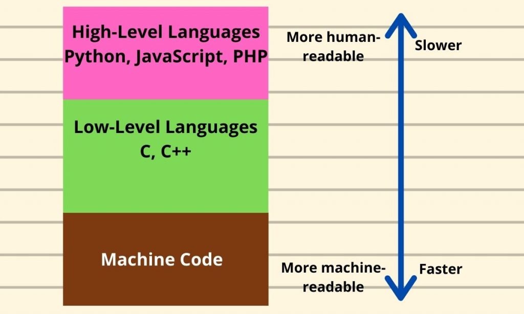
Note: Not all low-level, machine (Assembly) code is faster than high-level code. The primary reason that lower level coding tends to be faster is that it avoids a lot of the overhead (eg. garbage collection) involved in executing higher level code.
If you have done FIT2100 Operating Systems, this chapter would mostly be a refresher for you. It's intended to provide you with a crash course intro to operating systems theory so that you are capable of using low-level tools and implementing things like cache optimisations.
Computer Architecture
Nearly all modern computers are based on the Von-Neumann architecture which was introduced way back in 1945. Historically there have been 2 types of Computers:
- Fixed Program Computers: Their function is very specific and they couldn’t be reprogrammed, e.g. Calculators.
- Stored Program Computers: These can be programmed to carry out many different tasks, applications are stored on them, hence the name.
Modern computers are based on a stored-program concept introduced by John Von Neumann. In this stored-program concept, both software programs (code) and data (text, images, metadata, etc...) are stored in a separate storage unit called memory and are treated the same. This novel idea meant that a computer built with this architecture would be much easier to reprogram.
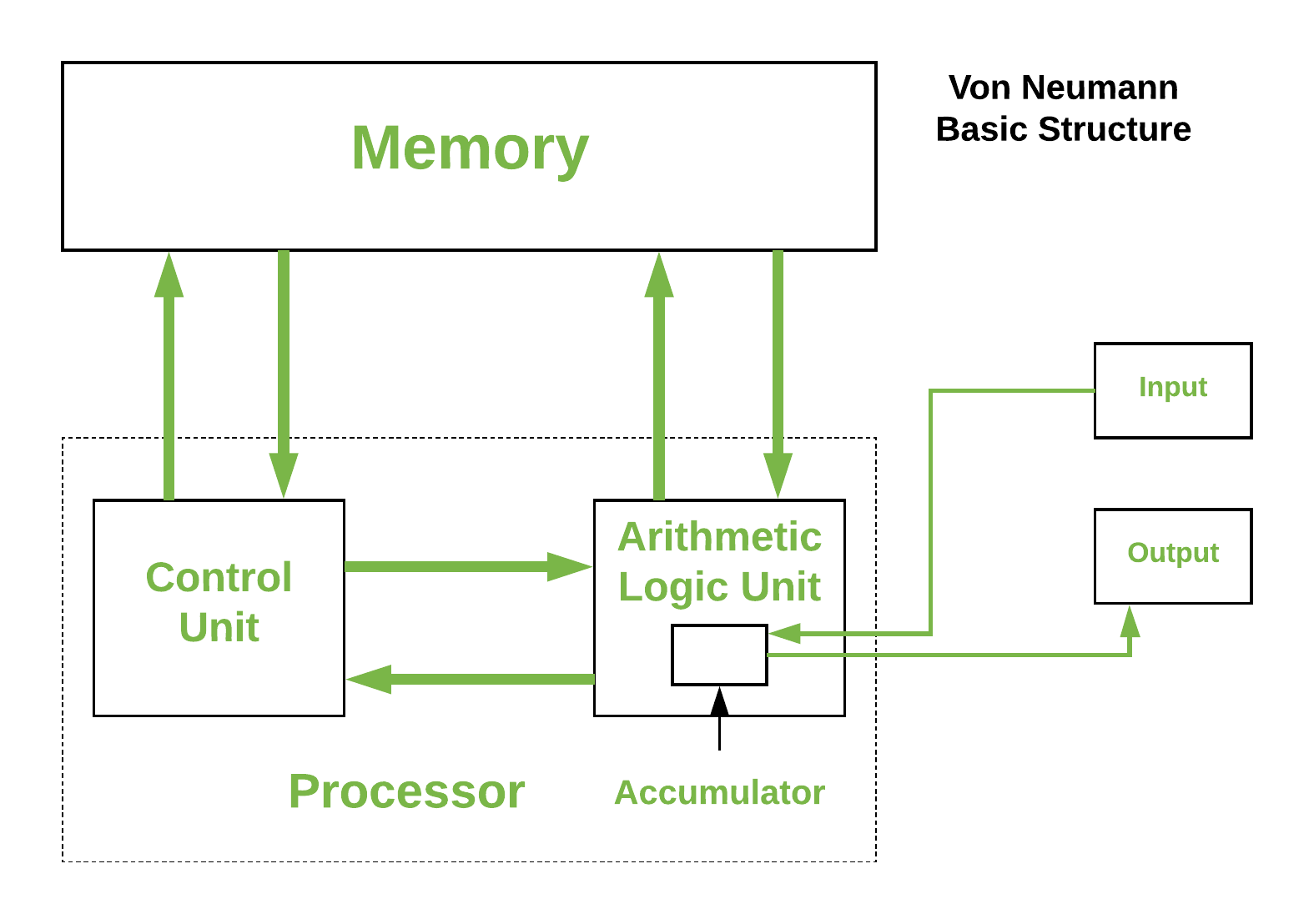
Central Processing Unit (CPU)
Hopefully everyone here knows what a CPU is and what it generally does. We've got a brief description of it's components and a lower level view of its hardware design to give you guys some relevant insight.
- Control Unit: A control unit directs all input and output flow, fetches code for instructions, and controls how data moves around the system. I think of it as the brains behind the CPU (the CPU of the CPU).
- Arithmetic Logic Unit (ALU): The ALU is the CPU component that handles all the calculations the CPU may need, e.g. Addition, Subtraction, Comparisons. It performs Logical Operations, Bit Shifting Operations, and Arithmetic operations.
Overview of Hardware Components
You don't need to remember everything here but as we pursue more hardware-related and low-level projects (Cluster Dev, potentially something in robotics...), these concepts are hopefully a good foundation for that.
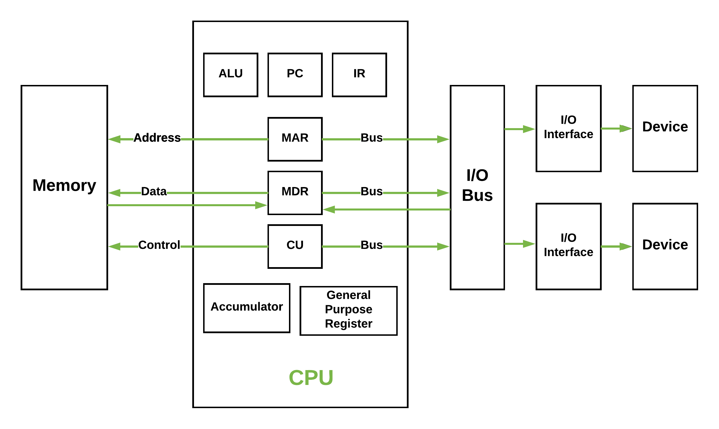
Registers
Registers refer to high-speed storage areas in the CPU. They are the most expensive but also the fastest unit of memory. The data processed by the CPU are fetched from the registers. There are different types of registers used in architecture:
- Accumulator: Stores the results of calculations made by ALU. It holds the intermediate of arithmetic and logical operatoins.it act as a temporary storage location or device.
- Program Counter (PC): Keeps track of the memory location of the next instructions to be dealt with. The PC then passes this next address to the Memory Address Register (MAR).
- Memory Address Register (MAR): It stores the memory locations of instructions that need to be fetched from memory or stored in memory.
- Memory Data Register (MDR): It stores instructions fetched from memory or any data that is to be transferred to, and stored in, memory.
- Current Instruction Register (CIR): It stores the most recently fetched instructions while it is waiting to be coded and executed.
- Instruction Buffer Register (IBR): The instruction that is not to be executed immediately is placed in the instruction buffer register IBR.
Buses
You can think of a bus as a group of tiny wires that carry data (64 tiny wires = 64 bit bus). Data is transmitted from one part of a computer to another, connecting all major internal components to the CPU and memory, by buses. Types:
- Data Bus: It carries data among the memory unit, the I/O devices, and the processor.
- Address Bus: It carries the address of data (not the actual data) between memory and processor.
- Control Bus: It carries control commands from the CPU (and status signals from other devices) in order to control and coordinate all the activities within the computer.
Input/Output Devices
Program or data is read into main memory from the input device or secondary storage under the control of CPU input instruction. Output devices are used to output information from a computer. If some results are evaluated by the computer and it is stored in the computer, then with the help of output devices, we can present them to the user.
Von Neumann bottleneck
Whatever we do to enhance performance, we cannot get away from the fact that instructions can only be done one at a time and can only be carried out sequentially. Both of these factors hold back the competence of the CPU. We can provide a Von Neumann processor with more cache, more RAM, or faster components but if original gains are to be made in CPU performance then a full hardware upgrade needs to happen. This is what motivates the use of parallel & distributed computing in HPC - it allows us to overcome this limitation without expensive hardware upgrades (details in later chapters).
Memory Heirarchy
It's very important that you understand these concepts as they go to the heart of memory-based optimisations in HPC. The main purpose behind designing a memory heirarchy is to use locality of reference to minimise access times as much as possible.
As you can see in the image below, there are multiple levels of memory with levels closer to the top (closer to the CPU) being smaller, more expensive but much faster than the ones to the bottom.

We can broadly divide this heirarchy into two:
- Primary Memory: This comprises Main Memory, Cache Memory & CPU registers and it's directly accessible by the processor.
- Secondary Memory: This is handled by external devices like Magnetic Disk, Optical Disk, and Magnetic Tape i.e. peripherals which are accessible by the processor via an I/O module and device driver.
Putting this heirarchy into perspective, we have some indicative stats below for each type of memory.
| Level | 1 | 2 | 3 | 4 |
|---|---|---|---|---|
| Name | Register | Cache | Main Memory | Secondary Memory |
| Size | <1 KB | <16 MB | <16GB | >100 GB |
| Hardware | D-latches | SRAM | DRAM | Magnetic |
| Access Time | 0.25-0.5ns | 0.5-25ns | 80-250ns | 500000 ns |
| Bandwidth | 20-100 GB | 5-15 GB | 1-5 GB | 20-150 MB |
| Managed by | Compiler | Hardware | Operating System | Operating System |
Pointers & Memory
Memory is one of the most important concepts in all of computing. Memory is the primary resource utilised in all programs and when it comes to large scale applications and programs it can easily be depleted. Being able to fine tune and control memory usage is one the best ways to optimize programs to ensure they are efficient and fast. However, this has the downside the programmer must control exactly how memory is used at all times increasing the cognitive complexity of a program which increases the likelihood that memory is misused programs leaking the resource. Many languages hide the details of memory usage and control to help reduce this cognitive complexity and reduce the risks of manual memory management. This can be done a variety of ways, from interpreters and virtual machines (Python, Java and C#) to using abstractions and semantics to hide the details while still allowing control when needed (C++, Rust) to straight up using a completely unique memory and data models (Haskell) however, C's memory model is the closest to how memory is truly laid out in hardware, largely because C and computer architecture have evolved together for so many decades. This is also because C is compiled end-to-end meaning source code is compiled directly into the machine language of the target machine not an intermediate bytecode or otherwise. This means that it is far simpler for C to model a machines memory architecture than create its own. This also simplifies C concept of memory greatly giving programmers the greatest level of control of memory (and other compute resources).
Brief Introduction into Memory
So what is memory? Memory; in its most abstract notion, is an 'infinite' sequence of fixed size cells. The size of these cells is (generally) 8-bits or a byte. On almost every computer, bytes are the smallest addressable unit of memory ie. they are the atoms of data. Any data you can build with a computer ultimately becomes some combination of bytes. But wait, what is a bit? A bit is a binary digit, thing of a regular (decimal) digit. It has 10 possible states (0..9) until it overflows and you need another digit (9 -> 10). A bit has only two possible states, 0 and 1.
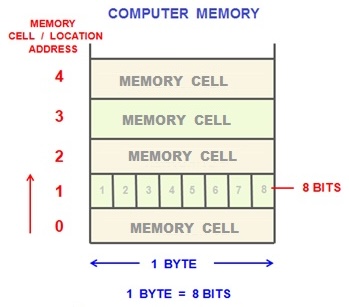
Bits are used as the extremely effective at modelling logical circuits where a wire is either on or off. Bits form the foundation for all of computing. However, inspecting and manipulating individual bits is tedious and only useful for small scale interactions. The goal of computing is to increase the computational power and thus reduce the time it takes to perform certain operations. This is why memory uses bytes. They are far easier to manipulate and are able to represent far larger data sets than a single bit (\(2^{8}=256\) combinations to be exact). However, while we can address individual bytes in memory this can be quite limiting in the number possible memory locations a CPU can address if we used a byte to represent the numerical address location of memory (a byte). Instead many machines use a machine word which represents the size of data a CPU is able to understand/read. The size of a word will correspond to the size of a CPU's registers, memory and IO buses and arithmetic manipulation hardware. Most machines have a word size of 64-bits or 8 bytes which dramatically increases the size of the instruction set used by a CPU, the amount of data it can transfer on buses and the amount of memory a CPU is able to address (\(2^{8}=256\) vs. \(2^{64}=1.844674407371 × 10^{19}\)). This is the largest integral value a machine is able to handle for most operations (ignoring specialised hardware).
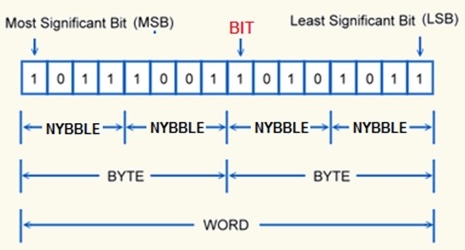
The Stack & Heap
Now, most computers do not give away all of their memory to a single application nor will memory used by an application allocate memory all from the same place. When a program executes the OS will allocates a small amount of memory to the memory for the instructions, constant data, meta data about the program and a small amount of free memory. This small amount of free memory is called the stack. Any local variables, function call stack and data created in a program are allocated to this part of the program automatically. However, the stack is quite small so when you need access to a large amount of memory you have to request it from the OS explicitly. The location where this OS owned memory is kept is called the heap (or free store). The heap is theoretically infinite in size allowing you to store large amounts of data however, you must remember to return it to the OS when you are done otherwise the memory will leak and the OS will loose track of it when your program finishes (or crashes).
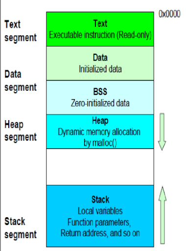
Besides, the stack and the heap you have the text and the data segment. The text segment would contain your executable instructions (your compiled C code) while the data segment has all initialised data. You also have a few other segments like BSS (Block Started by Symbol) which contains all uninitialised data and others not mentioned in the diagram above such as OS-reserved sections for Kernel code and data. If you ever wondered what RAM (main memory) actually looks like, well now you know.
What are Pointers?
So how do we refer to a memory. Fundamentally we need to be able to store the address of some piece data. This address is just some unsigned integer; with a bit size equivalent to a machine word. Using this address we then need to be able redirect access to the data held by at this memory address. We could just use a special integer type that corresponds to a machine word type and use this to store an address however, we often want to be able to access other pieces of data surround the data at the address we are storing thus we need to also be able to encode the type or size of the data whose address we are holding. This is because, while addresses all have the same size/width, it may own some data that is larger or smaller. Remember the smallest addressable machine location is a byte not a machine word. This construction we have described is called a pointer, simply because holds the location of some data ie. it points to some data. The type of a pointer is the type of the data being pointed to followed by an asterisks.
bool* pb;       //< Pointer to a bool
int* pi;        //< Pointer to an int
float* pf;      //< Pointer to a float
double* pd;     //< Pointer to a double
void* pd;       //< Pointer to a void
Note:
void*represents a polymorphic pointer type meaning it can point to data of any type and must be cast to the correct type on usage.
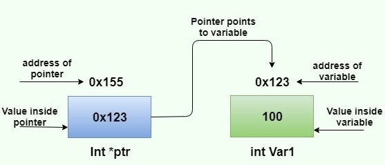
Obtaining Pointers
Every variable has an address regardless of whether they are created on the stack or the heap. So how do we get the address of a variable? There is a special operator we use called 'addressof' that returns the address of any variable. Its syntax is an ampersand (&) prefixed to any variable name.
#include <stdio.h>

int main()
{
    int a = 4;
    double b = 5.687;

    int* ap = &a;  //< can be assigned to a variable...

    printf("%d is at address: %p", a, ap);
    printf("%f is at address: %p", b, &b);  //< or used as a temporary

    return 0;
}
NULL
Sometimes a pointer does not own or point to anything. Instead of it pointing to data that might potentially not be ours to access we instead set the pointer to point to a compiler defined location called NULL. This is the empty address which prevents invalid access to it, usually by crashing though rather than undefined behaviour occurring. Always initialise or set a pointer to NULL if it does point to something and always check; when reasonable, if a pointer is NULL to prevent invalid access operations.
#include <stdio.h>

int main()
{
    int* p = NULL;
    printf("p points to: %p\n", p);

    int a = 4;
    p = &a;

    printf("p points to: %p\n", p);

    return 0;
}
Pointer Operations
Because pointers are just integral values we can perform regular integer arithmetic on them such as increment or decrement the address value to point to the next or previous memory location. You can also take the difference of two pointers to find the distance of two memory locations, add or take integral values from a pointer to jump a certain number of steps forward or backwards. The post important operation you can perform on a pointer is dereference it. This gives you access to the data being pointed to. Dereference involves using a prefix asterisks on the pointer variable. Any operation that is valid on the underlying data is valid on a dereference pointer.
#include <stdio.h>

int main()
{
    int a = 4;
    int* p = &a;

    printf("p points to: %p, with a value %d\n", p, *p);

    return 0;
}
Pointers to Pointers
Because pointers are just a numerical value they also have to store that numerical value. This value also has an address thus you are able to take the address of the pointer itself to obtain a pointer to a pointer. The type of a pointer to a pointer is the regular pointer type with additional asterisks suffixed to the type. This also means you can dereference the pointer to a pointer to obtainer the original pointers stored value which is the address of the original data. You can then dereference this pointer to get to the actual value. Additional dereferencing can be achieved by prefixing more asterisks to the pointer variable. This can be done for any number of pointer dereferences (pointer indirections).
#include <stdio.h>

int main()
{
    int a = 4;
    int* p = &a;
    int** pp = &p;

    printf("pp points to: %p, with a value %p\n", pp, *pp);
    printf("p points to: %p, with a value %d\n", p, *p);

    return 0;
}
Strings & Arrays as Pointers
Earlier, we kind of lied to you. We said that C supports array types. This is not entirely true. In reality arrays are just a pointer to a contiguous block of memory. In particular, the pointer points to the first memory location (element) of the array. The one difference is that arrays support the use of the subscript operator [] which performs a jump of n elements from the first element and automatic dereference of the pointer value giving you efficient access to the desired element. And because strings are just character arrays they are really just a pointer to the first element in the string literal ie. a char*. Almost always an array will decay into a pointer to the first element, particular when passing it to a function.
Note: Pointers still technically support
[]but unless it points to a contiguous block of data, the operation is mostly useless.
#include <stdio.h>

int main()
{
    char greeting[] = "Hello";
    char* farewell = "Goodbye";

    puts(greeting);
    puts(farewell);

    return 0;
}
Dynamic Memory
So far we have only used the stack for memory which has limited how much memory we can actually utilise. While this limit is implementation defined (differs depending on the platform and compiler) its also best not to fill up the stack with too much data that doesn't need to be there. Instead we can utilise the heap memory we discussed earlier, which is supplied by the OS. But how do we request this memory? For this we need to request the OS to allocate the necessary memory for our use and then allow us to access it. This is done by calling malloc(), which takes as input the size; in bytes, of the memory we wish to request from the OS and returns a void* to the allocated block. malloc() can be found in the <stdlib.h> header. Every called to malloc() must be paired with a call to free() which takes a pointer to a malloc() allocated block and returns the memory to the OS. Without free() the allocated memory will most likely not be freed by your program and thus leaks.
#include <stdio.h>
#include <stdlib.h>

int main()
{
    int* a = (int*)malloc(7 * sizeof(int));  //< Allocate 7 integers
    printf("a lives at: %p\n", a);

    for (int i = 0; i < 7; ++i)
        a[i] = i;

     for (int i = 0; i < 7; ++i)
        printf("%d\n", a[i]);

    free(a);
    return 0;
}
Note:
- Memory allocated by
malloc()is left in an uninitialised stake meaning whatever values that were left in that memory block remain ie. the junk that is help by the memory doesn't get cleared.- Because
malloc()just takes the number of bytes we want to allocate as a parameter we must calculate the total size of memory we need which depends on the size of an individual element ie. \(n × s\) where \(n\) is the number of elements we desire and \(s\) is the size of an individual element. We can use thesizeofoperator on a type name to get the size of that type.
Zero-Initialised Memory Allocation
Notice above we stated that malloc() returns a block of uninitialised memory but what if you want to memory that is initialised ahead of time. For this we use calloc(). This takes two parameters, the number of objects we wish to allocate and the size of each object. The memory block returned will have all of its bits initialised to 0.
#include <stdio.h>
#include <stdlib.h>

int main()
{
    int* a = (int*)calloc(4, sizeof(int));
    printf("a lives at: %p\n", a);

    for (int i = 0; i < 4; ++i)
        printf("%d\n", a[i]);

    free(a);
    return 0;
}
If you recall the previous subchapter,
calloc()allocates memory in the BSS segment instead of the heap/stack.
Reallocated Memory
We can also reallocate data to fit a larger or smaller amount. The elements from the old block will be copied to the new location until the new array is full or there are no more elements to copy. realloc() my not actual allocate memory in a new locating if there is free space next to the existing array. realloc() also works like malloc() where the new memory is left uninitialised. realloc() takes two parameters, the old pointer address and the new size.
#include <stdio.h>
#include <stdlib.h>

int main()
{
    int* a = (int*)malloc(4 * sizeof(int));
    printf("a lives at: %p\n", a);

    for (int i = 0; i < 4; ++i)
        a[i] = i;

    for (int i = 0; i < 4; ++i)
        printf("%d, ", a[i]);

    a = (int*)realloc(a, 7);
    printf("\na lives at: %p\n", a);

    for (int i = 0; i < 7; ++i)
        printf("%d, ", a[i]);

    free(a);
    return 0;
}
Note:
- Any memory allocated by
malloc(),calloc()orrealloc()must be returned to the OS by a call tofree().
General Memory Utilities
C features a few byte based memory operations that is able to set, compare and copy data. These are memset(), memcmp() and memcpy() respectively. These memory utilities are found in the <string.h> header.
memset()
memset() takes an input pointer that you wish to modify, an int value which is narrowed to an unsigned char; such that each byte of the input memory is set this value, and a count for the number of bytes affected. This is not to be confused will a general fill algorithm as this function writes to individual bytes not to individual elements in a memory block.
#include <stdio.h>
#include <stdlib.h>
#include <string.h>

int main()
{
    int* a = (int*)calloc(4, sizeof(int));

    for (int i = 0; i < 4; ++i)
        printf("%d, ", a[i]);

    puts("");

    memset(a, (unsigned char)1, 6);

    for (int i = 0; i < 4; ++i)
        printf("%d, ", a[i]);

    free(a);
    return 0;
}
memcmp()
memcmp() will lexicographically compare the bytes of two input pointers up until the specified count. Returning a negative value if the bytes passed as the left argument is greater than the right, 0 if they are the same or a positive value of the right is greater then the left.
#include <stdio.h>
#include <stdlib.h>
#include <string.h>

int main()
{
    int* a = (int*)calloc(4, sizeof(int));
    int* b = (int*)calloc(4, sizeof(int));

    for (int i = 0; i < 4; ++i)
        printf("%d, ", a[i]);

    puts("");

    for (int i = 0; i < 4; ++i)
        printf("%d, ", b[i]);

    puts("");

    int cmp = memcmp(a, b, 4);
    printf("a = b: %d\n", cmp);

    memset(a, (unsigned char)1, 6);

    cmp = memcmp(a, b, 4);
    printf("a = b: %d\n", cmp);

    free(a);
    free(b);
    return 0;
}
memcpy()
memcpy() is probably the most useful as it allows you to efficiently copy the bytes directly from one memory block to another. It takes two input pointers with the first be the destination and the second being the source. it also takes a count for the number of bytes you want to copy.
#include <stdio.h>
#include <stdlib.h>
#include <string.h>

int main()
{
    int* a = (int*)calloc(4, sizeof(int));
    int b[] = { 1, 2, 3, 4 };

    for (int i = 0; i < 4; ++i)
        printf("%d, ", a[i]);

    puts("");

    for (int i = 0; i < 4; ++i)
        printf("%d, ", b[i]);

    puts("\n");

    memcpy(a, b, 4 * sizeof(int));

    for (int i = 0; i < 4; ++i)
        printf("%d, ", a[i]);

    puts("");

    for (int i = 0; i < 4; ++i)
        printf("%d, ", b[i]);

    puts("");

    free(a);
    return 0;
}
Note: If you access more bytes than what is allocated to a pointer using any of these algorithms or even directly will cause undefined behaviour which might (hopefull) crash the program or lead to consequences that are very hard to trace. Don't do it.
Dynamic String Utilities
Since operating on strings is so common their are more specific string manipulation functions available. These allow you to more easily work with character arrays and manipulate them in the way you would expect. These functions can be found in the <string.h> header.
strlen()
Obtains the length of a null-terminating string, not including the null-terminated character. It is undefined if the string is not null-terminated.
#include <stdio.h>
#include <string.h>

int main()
{
    char c[] = "Hello";

    printf("sizeof(c) = %zu\n", sizeof(c));
    printf("strlen(c) = %zu\n", strlen(c));

    return 0;
}
strcmp()
Compares to strings lexicographically, same manner as memcmp(). The return value is also an int with a negative value meaning the left is greater than the right, 0 meaning they are the same and a positive value meaning the right is greater than the left.
#include <stdio.h>
#include <string.h>

int main()
{
    char a[] = "Hello";
    char b[] = "Hello";

    int cmp = strcmp(a, b);
    printf("a = b: %d\n", cmp);

    a[1] = 'E';
    cmp = strcmp(a, b);
    printf("a = b: %d\n", cmp);

    return 0;
}
strcpy()
Allows you to efficiently copy the characters from one string to another including the null-terminator. The first argument is the destination adn the second is the source. Returns a copy of the destination pointer.
#include <stdio.h>
#include <string.h>

int main()
{
    char a[] = "Hello";
    char b[strlen(a) + 1];  //< +1 to accommodate the null-terminator

    printf("%s\n", a);
    printf("%s\n\n", b);

    strcpy(b, a);

    printf("%s\n", a);
    printf("%s\n", b);

    return 0;
}
strcat()
Concatenates two strings by appending the second string to the end of the first.
#include <stdio.h>
#include <string.h>

int main()
{
    char a[13] = "Hello";
    char b[] = " World!";

    printf("%s\n", a);
    printf("%s\n\n", b);

    strcat(a, b);

    printf("%s\n", a);
    printf("%s\n", b);

    return 0;
}
Structures & Macros
Now let's cover some more advanced C language features before delving into operating system concepts.
Structures
So far we have only been able to to manipulate primitive data types and collections of a single type but what if we want to manipulate and store data that is of different types. This is where structures come in. Structures are used to hold data of different types in a compact format. Structures are created using the struct keyword paired with a unique name followed by a brace scope of variable declarations. To then create a variable of the structure type you again use the struct keyword and the structures type name followed by a variable name. You can then initialise the fields using a comma separated list, enclosed in braces where each element is the desired value for initialising the field of the structure. The fields are then accessed using the variable and the member access operator (.) paired with the field's name.
#include <stdio.h>

struct A
{
    int i;
    double d;
    char* c;
};

int main()
{
    struct A a = { 5, 576.658, "Hello" };
    printf("%d\n", a.i);
    printf("%f\n", a.d);
    printf("%s\n", a.c);

    return 0;
}
Note:
- Structures do not support methods.
- Elements in a structure a layed out contiguously ie. each element is right next to each other.
- The size of a structure can be obtained normally using
sizeof.
Macros & The Preprocessor
Sometimes we need to control how source code is compiled, enable certain parts of the source code while disabling other parts. How do you do this? This is done using macros in C. Macros are compile time expressions that are executed by a part of the compiler called the preprocessor.
What is a macro?
Macros are expressions that are evaluated and removed from the final source code. They are created using a # followed by a macro identifier. One macro we have used consistently throughout this book is the #include macro which is used to copy the source code from header files into other source and header files. Macros in C mostly perform in-source text replacement.
Note: Conventionally, macro symbols (names) are written in all uppercase to prevent conflation with regular source code.
#define & #undef
The most common and general macro is the #define macro. This allows you to define a symbol that will be replaced with its definition during the compilation phase. #undef can be used to undefine a symbol so that its usage is ignored. Names, value, types and even function-like entities can be defined and undefined using #define and #undef.
#include <stdio.h>

#define INT int

#define ADD(x, y) x + y

int main()
{
    INT i = 5;  //< Ok
    printf("%d\n", i);
    printf("%d\n", ADD(i, 2));

    #undef INT
    // INT a = 4;  //< Compile time error

    return 0;
}
Note: Even though you can define function-like entities using macros I would highly recommend against it in 99% of cases as it is nearly impossible to debug as the macros are expanded and removed very early on in the compilation of a program.
Include Guards
One common use of macros is for include guards. These are valueless macros that are defined once for a header file and only expose the contents of the header file if the macro is not defined. This prevents headers from being included twice and causing a redefinition or duplication error. How does this work? Essentially, when a header is first encountered, a macro is checked. If it is not defined we then define it and define the rest of the contents of the header. If it was already defined then the header is 'empty'. This stops the contents of headers being imported multiple times or as a transitive dependency.
#ifndef HEADER
#define HEADER

/// Headers contents

#endif  /// HEADER
Defining Macros from the Command Line
Macros are able to be defined from the command line through the compiler. Many compilers support a -D and -U fag which can define and undefine macros in source code respectively. These are typically used to control macros similar to header guards which control which parts of a codebase are defined eg. for different OS or graphical backends.
# Forces in to be defined
gcc -o main -DUSE_WINDOWS_INT main.cpp
#if, #elif, #else, #ifdef, ifndef and #endif
The other common class of macros is the control flow macros. These can control which parts of the source code are visible to the compiler thus which parts are compiled. They can be used just like regular control flow using predicates to determine the correct part of the codebase to use. However, they often are used with empty macros which are control from the command line to easily control which parts of the code we wish to compile. The #ifdef and #ifndef macros are slightly different in the sense that they check if other macros are defined as apposed to checking a predicate. All control flow macros must end in #endif for the final macro expression to help denote the end of a macros scope as macros do not use braces.
#include <stdio.h>

#if ADD
    int op(int a, int b)
    { return a + b; }
#elif SUB
    int op(int a, int b)
    { return a - b; }
#else
    int op(int a, int b)
    { return a * b; }
#endif /// ADD

int main()
{
    printf("%d\n", op(5, 6));

    return 0;
}
Try it yourself. Write up the following code and see how using the
-Dflag when compiling it changes the outcome.
#pragma
The final macro worth mentioning is the #pragma macro. This macro is special is it is used by compilers and libraries to implement specific and unique features to their platform. In essence these are non-portable and non-standard macro that are specific to the platform you are targeting or compiler you are building with. A common #pragma directive in many C compilers in the #pragma once directive which is designed to replace the need for header guard.
#pragma once

/// Header's content
Introduction to Linux
Linux is a freely available open-source operating system built by Linux Torvalds back in 1991. It's based off of Bell Lab's development of Unix in the 1970s which also forms the basis of Android and MacOS. It's an extremely popular operating system, especially for servers (nearly all nodes in M3 use Linux). We will be learning about it and using it to gain both low-level programming skills and an understanding of Operating Systems theory.
There are various implementations (distributions) of Linux. We won't go into detail on them but here's a comparison of some of the popular ones.
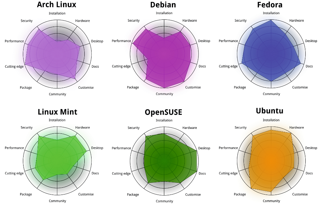
You can think of Linux as having 3 layers or components. Here they are from the highest to the lowest level (how removed they are from the hardware):
- System Libraries: System libraries are special functions or programs using which application programs or system utilities access the Kernel’s features. This is the topmost layer of the operating system. It allows access to the deeper parts of the machine without exposing them to direct user access. One such example for Linux and other Unix-like operating systems is
unistd.hwhich provides C functions to access the POSIX (Portable Operating System Interface) API. - Kernel: The kernel is the core part of Linux. It is responsible for all major activities of this operating system. It consists of various modules which are all hidden and protected from the user. The only way that a user can access the kernel is through the system library. I encourage you all to check out the Linux kernel code on GitHub (you can see Linus still actively approving all the PRs into master).
- Device Drivers (Kernel Modules): If you wondered how an operating system actually controls the hardware this is how they do it. They use device drivers/kernel modules which are software programs written to act as an interface between the OS kernel and the device's firmware.
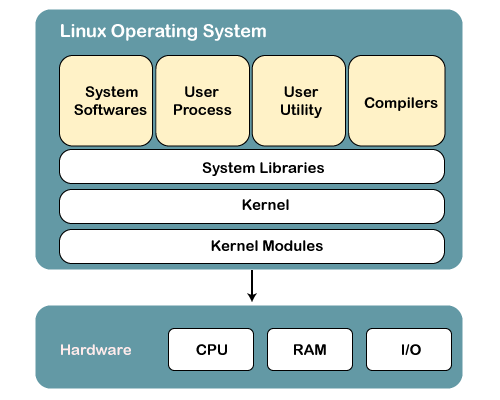
What does an operating system actually do?
Pretty much all interactions you have with your machine is facilitated by an operating system. I find it useful to break it down into 2 functional areas - compute (algorithms/processes/dynamic stuff) and storage (data structures/memory/static stuff).
Compute
The operating system is what ultimately controls the CPU. Time on the CPU is a scarce resource for user applications that need to get code/instructions executed as quick as possible. Hence why compute is considered a "resource" and the OS is responsible for the fair and efficient allocation of this and all resources.
Some more terminology - a program is a file with some non-executing (static) code while a process can be thought of as a live program that's being executed on the CPU.
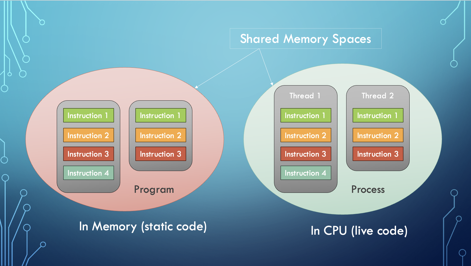
Operating systems have to enable the creation of new processes, schedule them time on a CPU, manage and keep track of processes while also handling their completion. To do this there are a lot of attributes, structures and behaviours implemented by the Linux kernel.
Process Characteristics & Attributes
A process has the following attributes:
- Process Id: A unique identifier assigned by the operating system.
- Process State: Can be ready, running, etc.
- CPU registers: Like the Program Counter (CPU registers must be saved and restored when a process is swapped in and out of the CPU)
- Accounts information: Amount of CPU used for process execution, time limits, execution ID, etc
- I/O (input/output) status information: For example, devices allocated to the process, open files, etc
- CPU scheduling information: For example, Priority (Different processes may have different priorities, for example, a shorter process assigned high priority in the shortest job first scheduling)
A process is in one of the following states at any given time:
- New: Newly Created Process (or) being-created process.
- Ready: After the creation process moves to the Ready state, i.e. the process is ready for execution.
- Run: Currently running process in CPU (only one process at a time can be under execution in a single processor)
- Wait (or Block): When a process requests I/O access.
- Complete (or Terminated): The process completed its execution.
- Suspended Ready: When the ready queue becomes full, some processes are moved to a suspended ready state
- Suspended Block: When the waiting queue becomes full.
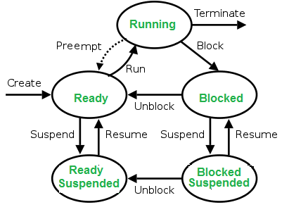
Context Switching
The process of saving the context of one process and loading the context of another process is known as Context Switching. In simple terms, it is unloading a running process into the ready state in order to load another ready process into the running state.
When Does Context Switching Happen?
- When a high-priority process comes to a ready state (i.e. with higher priority than the running process).
- An Interrupt occurs (some I/O device tells the kernel that it needs CPU time).
- User and kernel-mode switch.
- Preemptive CPU scheduling is used (context switches at regular time intervals).
There is a lot more involved in how compute is managed by the OS (eg. process scheduling, threading, etc...) which will be covered in a later chapter.
Storage
If you recall chapter 3.1, this area can be further subdivided into two - temporary storage (main memory i.e. RAM) and permenant storage (hard drives and SSDs).
Linux File Systems
As you all know, computers manage the permenant storage of information using a system of files and directories. The Linux file system is a multifaceted structure comprised of three essential layers. At its foundation, the Logical File System serves as the interface between user applications and the file system, managing operations like opening, reading, and closing files. Below this layer, the Virtual File System facilitates the concurrent operation of multiple physical file systems, providing a standardized interface for compatibility. Finally, the Physical File System is responsible for the tangible management and storage of physical memory blocks on the disk, ensuring efficient data allocation and retrieval. Together, these layers form a cohesive architecture, orchestrating the organized and efficient handling of data in the Linux operating system.
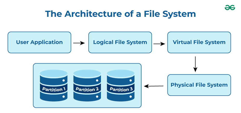
Paging & Memory Allocation
Paging is a memory management technique in operating systems that enables processes to access more memory than is physically available. The system improves performance and resource utilization using virtual memory. A process has access to the pages it needs without waiting for them to be loaded into physical memory. The technique stores and retrieves data from a computer's secondary or virtual storage (hard drive, SSD, etc.) to the primary storage (RAM).
When a process tries to access a page that is not in RAM, the OS raises a page fault and brings in the page from virtual memory.
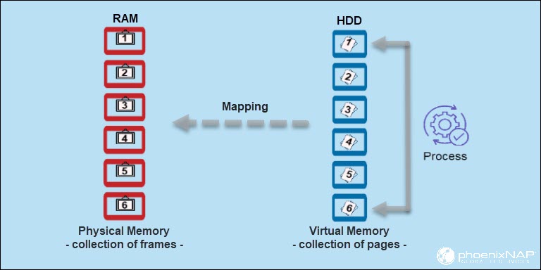
Paging improves the efficiency of memory management. By dividing memory into pages, the operating system moves pages in and out of memory as needed. Keeping only the frequently used pages reduces the number of page faults, which improves system performance and responsiveness. This is a key HPC optimisation concept known as locality of reference.
Cache Optimisation
A lot of you must be familiar with the concept of caching. It basically means storing data temporarily in an easily accessible place in order to be more efficient when accessing it. Nearly all modern PCs use caches for efficiency. If you recall the memory heirarchy in chapter 3.1, caches sit between CPU registers and main memory (RAM) in terms of speed and cost. There are usually 3 levels of caches (depending on computer architecture) - L1, L2 and L3 with L1 being the smallest, most expensive, fastest and closest to the CPU.

In the above figure, you can see that the CPU wants to read or fetch the data or instruction. First, it will access the cache memory as it is near to it and provides very fast access. If the required data or instruction is found, it will be fetched. This situation is known as a cache hit. But if the required data or instruction is not found in the cache memory then this situation is known as a cache miss.
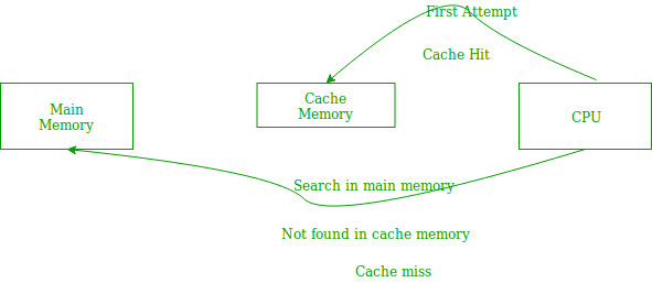
The aim is to store data that any given process is likely to access in the future, in the cache. Cache optimisation involves minimising the no. of cache misses while maximizing cache hits. The benefits are obvious - reduced memory access times resulting in a faster program. Cache optimisation is done by implementing locality of reference and there are two localities:
-
Temporal locality is when current data or instruction that is being fetched frequently may be needed soon. It's based on the same assumption that if a program is accessing the same location (using pointers) again and again then it's likely to access it in the immediate future as well.
-
Spatial locality, on the other hand, assumes that memory addresses that are closer to currently accessed addresses are more likely to be accessed again.

Accessing the Kernel's API
As mentioned earlier, user space programs (code that a programmer writes for an application/script) will need to use a system library to access the kernel and it's lower-level functionality. For Linux, the main library is unistd.h which only runs on POSIX-compatible (Unix-like) operating systems and unfortunately Windows is not one of them. To get around this, we will be using a Docker container with an Ubuntu image.
Note: You can also use WSL or launch an Ubuntu VM to get
unistd.hworking. But it's useful to know Docker in case you ever need to replicate the same environment and avoid dependency-related bugs while working in teams or if you need to do container-based deployments.
VMs & Containers
In order to succeed in HPC, you will need to know how distributed computing works. Virtual machines and containers are a way of doing distributed computing and we'll give a decent introduction to them here. They help in a lot of scenarios both in your MDN work and in the real-world by allowing you to manage dependencies (eg. for a custom benchmarking script) and deploy an application into a server (eg. for a public HPC visualisation website).
What is a virtual machine (VM)?
A virtual machine is not a physical machine. It’s a file that replicates the computing environment of a physical machine. It’s similar to how virtual reality (VR) environments replicate the real world. VR isn’t a physical space; it’s a virtual imitation. Still, we can perform real-world functions in VR, such as exploring and interacting with objects. Instead of imitating video game functions, virtual machine software emulates computer system functions i.e. the operating system. To achieve this VMs use a technology called virtualisation as shown below.
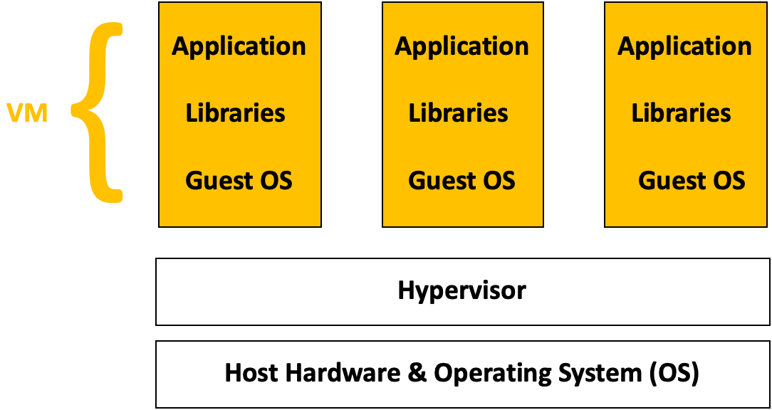
At the base, you have the host hardware and OS. This is the physical machine that is used to create the virtual machines. On top of this, you have the hypervisor. This allows multiple virtual machines, each with their own operating systems (OS), to run on a single physical server.
VMs have a few downsides, though, which containers address. Two downsides particularly stand out:
- VMs consume more resources: VMs have a higher resource overhead due to the need to run a full OS instance for each VM. This can lead to larger memory and storage consumption. This in turn can have a negative effect on performance and startup times of the virtual machine.
- Less portability: VMs are typically less portable due to differences in underlying OS environments. Moving VMs between different hypervisors or cloud providers can be more complex.
There are a few upsides though and they mostly apply if you need better isolation/security or more control over low level things that containers don't give you access to. If you want to learn how to launch and use VMs, it's covered in ARDC's Nectar Cloud starter tutorial series. You can also check out other cloud platform providers like Amazon Web Services (AWS) and Microsoft Azure.
What is a container?
A container is a lightweight, standalone, and executable software package that includes everything needed to run a piece of software, including the code, runtime, system tools, and libraries.
Containers are designed to isolate applications and their dependencies, ensuring that they can run consistently across different environments. Whether the application is running from your computer or in the cloud, the application behaviour remains the same.
Unlike VMs which virtualise the hardware, containers virtualise the operating system. This simply means that a container uses a single OS to create a virtual application and its libraries. Containers run on top of a shared OS provided by the host system.
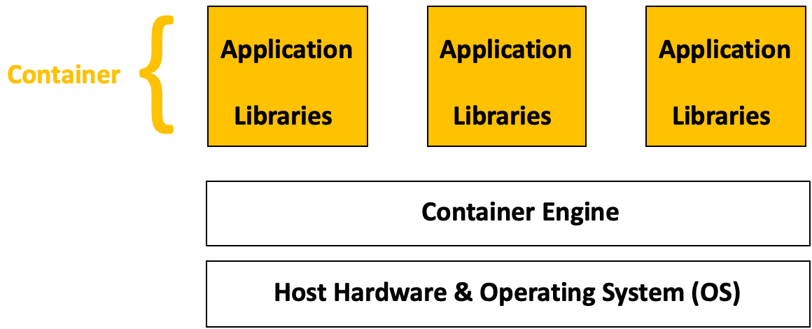
The container engine allows you to spin up containers. It provides the tools and services necessary for building, running, and deploying containerised applications. If you ever had the problem below, containers are a life saver.
Docker
As you might know, Docker is an open-source containerization platform by which you can pack your application and all its dependencies into a standardized unit called a container. Let's clarify some Docker terminology,
- Docker Image: An image is an inert, immutable, file that's essentially a snapshot of a container. Images are created with the build command, and they'll produce a container when started with run. Images are stored in a Docker registry such as registry.hub.docker.com.
- Docker Container: To use a programming metaphor, if an image is a class, then a container is an instance of a class—a runtime object. Multiple containers can run from the same image simultaneously.
- Docker Daemon: The Docker daemon (
dockerd) listens for Docker API requests and manages Docker objects such as images, containers, networks, and volumes. - Docker Client: The Docker client (
docker) is the primary way that many Docker users interact with Docker. When you use commands such asdocker run, the client sends these commands todockerd, which carries them out. - Docker Desktop: This is an easy-to-install application for your Mac, Windows or Linux environment that enables you to build and share containerized applications and microservices.
Docker Architecture
Docker uses a client-server architecture. The Docker client talks to the Docker daemon, which does the heavy lifting of building, running, and distributing your Docker containers.
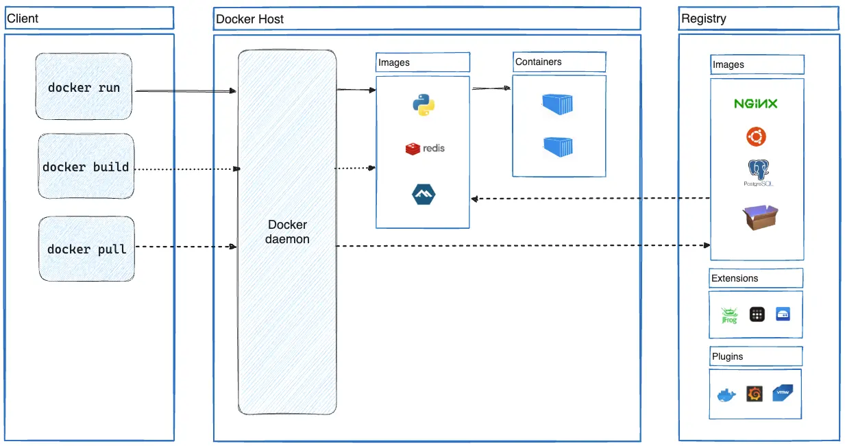
Go through this guide to download and install Docker. If you'd like to learn more about it's functionality and how to work with it, check out their documentation website. We will go through the basics of how Docker and it's CLI (command-line interface) works to get you started.
Launch Docker Daemon
Before we get started it's important to make sure the Docker daemon (background process that manages Docker) is running. In order to launch it, go to your docker desktop app and run it.
Check Version
If you want to know what version of Docker you're running, use this command. It's also a useful command for checking if you've correctly installed and launched Docker.
docker version
More Info
For more info about installation and the no. of Docker objects (images, containers, networks, etc...) use this command.
docker info
List Containers
To list all running containers use the command below. To include ones that are not currently running as well, use the command with the -a flag.
docker ps
List Images
Likewise to list all images you have downloaded, use the command below.
docker images
Download Image
Similar to GitHub, if you want to download an image you "pull" it from the Docker registry.
docker pull nginx
This command will pull the latest image of nginx (a HTTP server) from Docker Hub's registry.
Stop/Remove Containers & Images
To stop a running container and to remove containers and images you use the following commands. For stopping a container:
docker stop {container_name_or_id}
For removing a container:
docker rm {container_name_or_id}
For removing an image:
docker rmi {image_name_or_id}
Start and work with containers
To create a new container from an image after you've pulled it, use:
docker run {image_name_or_id}
After the container is created, you can start (launch) it by running:
docker start {container_name_or_id}
If you want to actually run commands inside, for example - to open a Bash terminal:
docker exec -it {container_name_or_id} bash
The
-itflag specifies to run it in interactive mode-iand to allocate a psueo-TTY-t.
Advanced Docker Concepts
This is a little out of scope for the training book but if you want to build your Docker image, you will have to use docker build. Other docker functionality to be aware of:
- For managing a lot of containers using declarative config files - Docker Compose
- To find and share container images (like GitHub) - Docker Hub
- If you want your containers to talk to each other - Docker Network
- For image scanning, analysis and security-related things - Docker Scout
There are a bunch of other extensions and software that's designed to work with Docker that are not mentioned here. Important takeaway here is that if you ever have to manage dependencies and/or work across teams doing that (which you will definitely have to do in an advanced HPC project) - containers make your life a lot easier. This is also the case if you want to deploy and scale any web service for which you can use something like Kubernetes. Container-based deployments are becoming more and more popular due to how lightweight and flexible they are compared to traditional virtual machines.
Bash Commands & Scripts
Bash (the Bourne-Again SHell) is a terminal that allows you to enter commands and write scripts in order to access the Kernel's functionality. It's similar to system libraries (for programming) and the GUI (for non-IT people) in that it's a way to navigate your operating system and use the services that it provides, i.e. it's your kernel's interface. Bash in particular was created in the late 1980s as part of the GNU project and it was intended to replace the Bourne shell, hence Bourne-again shell.
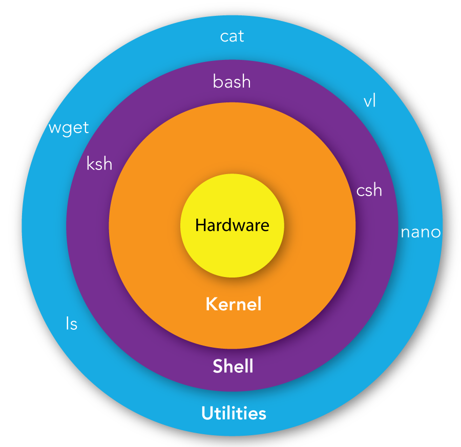
Basic Linux Commands
These commands will be your bread and better whenever you can't access the GUI or the GUI doesn't provide enough functionality, which will be the case for a lot of HPC work. You will have to be comfortable using these commands, writing Bash scripts and navigating the Linux environment.
| Command | Function |
|---|---|
pwd | prints current directory |
ls | prints list of files / directories in current directory (add a -a to list everything, including hidden files/directories |
mkdir | makes a directory |
rm <filename> | deletes filename. add -r to delete directory. add -f to force deletion (be really careful with that one) |
cd <directory> | move directory. |
vim or nano | bring up a text editor |
cat <filename> | prints contents of file to terminal |
echo | prints whatever you put after it |
chmod <filename> | changes permissions of file |
cp | copy a file or directory |
mv <filename> | move or rename file or directory |
grep | Search for a pattern in files |
touch <filename> | Create an empty file in current dir |
Note:
.and..are special directories..is the current directory, and..is the parent directory. These can be used when using any command that takes a directory as an argument. Similar to these,~is the home directory, and/is the root directory. For example, if you wanted to copy something from the parent directory to the home directory, you could docp ../<filename> ~/, without having to navigate anywhere.
Piping
If you want to use the output of one command as input to another, you can simply "pipe" it to the other command. For example, if you want to search your directory to find a file named somefile.someextension you can do this:
ls | grep somefile.someextension
Bash Scripts
Bash is both a command line interface and a scripting language. Bash scripts are useful for automating tasks that you do often, or for running a series of commands that you don't want to type out every time.
In terms of use, Bash can encapsulate any command you would normally run in the terminal into a script that can be easily reused. For example you could have a script that automatically navigates to a directory and activates a virtual environment, or a script that compiles and runs a C program.
The basic syntax of a bash file is as follows:
#!/bin/bash

# This is a comment

echo "Hello World"
We can save this file as hello.sh and run it using the following command: source hello.sh. This will print Hello World to the terminal.
Let's walk through the file. The first line is #!/bin/bash. This is called a shebang, and it tells the system that this file is a bash script. The second line is a comment, and is ignored by the system. The third line is the actual command that we want to run. In this case, we are using the echo command to print Hello World to the terminal.
Bash can do a lot more, including basic arithmetic, if statements, loops, and functions. If you want to learn more about bash, you can find a good tutorial here.
The main things we need to be able to do are to run executables and files. We do this the exact same way as if manually running them in the terminal. For example, if we want to run a python script, we can do the following:
#!/bin/bash

# This will run hello.py using the python3 executable
python3 hello.py
If we want to compile and then run a C program, we can do the following:
#!/bin/bash

# This will compile hello.c and then run it
gcc hello.c -o hello
./hello
Processes & Threads
As introduced earlier, when computer runs a program, your source code is loaded into RAM and process is started. A process is a collection of code, memory, data and other resources. A process runs in a unique address space. So Two processes can not see each other’s memory.
A thread is a sequence of code that is executed inside the scope of the process. You can (usually) have multiple threads executing concurrently within the same process. Threads can view the memory (i.e. variables) of other threads within the same process
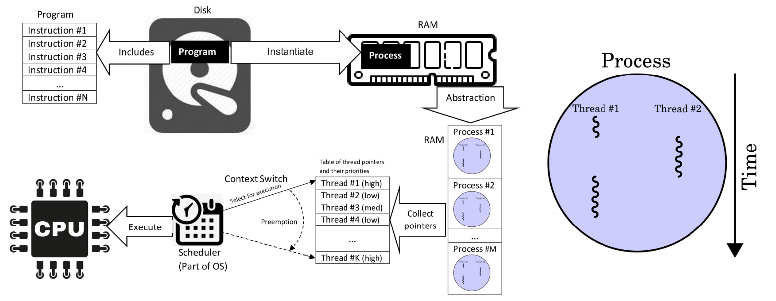
A multiprocessing system has more than two processors, whereas multithreading is a program execution technique that allows a single process to have multiple code segments.
Bash Process Management
There are several commands in Bash for process management. Following are some commonly used commands:
| Command | Purpose |
|---|---|
ps | Lists all processes in the system. |
top | Tracks the running processes on the system and provides real-time information. |
kill | Terminates a running process by sending a signal. |
pkill | Sends a termination signal to a process. |
jobs | Lists all the running jobs (tasks) in the system. |
fg | Moves a background process to the foreground. |
bg | Restarts a stopped process to run in the background. |
nice | Adjusts the priority of a process. |
renice | Changes or adjusts the priority of a running process. |
free | Displays the status of RAM. |
df | Shows the disk management of the system. |
As you might have noticed if you ran ps or top, each Bash command spawns (creates) a process. That's because all of these commands are just executable binary files that are software programs (exactly the same as compiled C code) that you can find in one of your system directories.
Pro-Tip: The
-oflag with thepscommand allows you to specify the columns to list for processes. For example, to list the process ID, nice score and command name for each process useps -o pid,ni,cmd.
Signals
In Linux, a signal is a notification sent to a process to indicate an event. Typically it is triggered by the operating system, hardware, or other processes in order to signify various events, including process termination, user interrupts, errors, and system events. A unique identifier represents each signal and has predefined behaviors associated with it.
To get a list of all signals in Bash use:
kill -l
Which should give you an output similar to below,
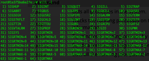
From the above you can see that to kill/terminate a process (SIGKILL), you need to use signal 9. To kill a process you can use the command kill -9 <pid>. If you need to kill a deadlocked/non-responsive process on a HPC node with no GUI, this would come in handy.
Process Priorities
A process's priority determines when and how much CPU walltime it gets. This is also the case in Slurm or any other multi-user/multi-process system with a scheduler so it's useful to know how process priorities work.
Managing a process’s priority involves altering the order of priority in which processes are executed by the system. By setting the priority, you can make sure that the most important tasks get the most CPU time to receive the necessary system resources compared to the less important tasks. Some common aspects of prioritizing processes:
Process Priority Range
The priority value of a process is known as the ‘nice value’ that typically ranges from -20 to 19, where -20 indicates the highest priority and 19 indicates the lowest priority. By default, the processes launched from the terminal have a zero (0) value of priority. The negative values (-20 to 0) are reserved for real-time tasks while the positive values (0-19) are for normal user processes or tasks.
Using “nice” Command
The nice command starts a process with a specified priority level. It assigns a lower priority to a process as the lower the nice values, the higher the priority. The syntax to use the nice command is nice -n <priority> <command>.
Using “renice” Command
The renice command modifies and adjusts the priority of a process that is already running. This command either increases or decreases the priority of a process based on the specific value. The syntax to use the renice command is renice <priority> -p <pid>.
Decreasing priority can be done by any user in the system but the priority can only be increased by the process owner or the super user (root).
Scheduling Algorithms
As you might've noticed, your computer runs a large amount of processes (around 500+) at any given time. Most of them are system utilities and kernel processes that you don't really have access to but a lot of them involve applications you opened or commands you've typed into your terminal. Even though most modern CPUs have 8+ cores so they can run 8 processes/execute 8 threads at the same time, there's obviously a need to queue these processes and schedule them time on the CPU in an orderly manner. In order to do this, there are a variety of scheduling algorithms.
Knowing these scheduling algorithms also helps you understand how scheduling works in a HPC cluster. This is important if you're involved in a HPC project that builds, manages and/or analyses a cluster from an admin perspective and also as a user that's wondering why their job (process) isn't getting much time on compute nodes.
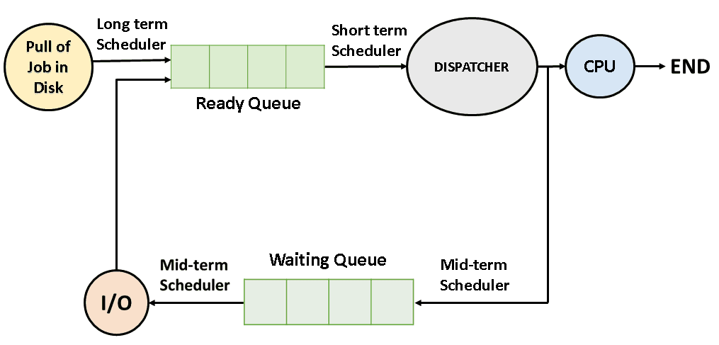
Hopefully the diagram above is self-explanatory at this point. There's a lot of implementation details involved in the specific type of scheduler you're using (i.e. Linux Kernel) but we will focus on high-level concepts that are also generalisable to HPC cluster schedulers.
Terminology
Before we start there's some terminology to clarify and define:
- Preemptive Scheduling: This is a scheduling policy where a process running in a CPU can be interrupted (blocked/stopped) and moved to the ready state while another process starts running on the CPU.
- Wait Time: Wait time refers to the period during which a process remains in the ready queue, waiting for CPU execution.
- Arrival Time: Arrival time is the moment when a process enters the ready state and becomes eligible for execution.
- Burst Time: Burst time (execution/wall time) is the total time taken by a process to execute on the CPU.
- Turnaround Time: Turnaround time is the total time taken for a process to complete its execution from submission to exit. It includes the waiting time, execution time, and any other overhead (such as context switching). Turnaround time is a crucial metric for evaluating scheduling algorithms and system performance (for both PCs & HPC cluster).
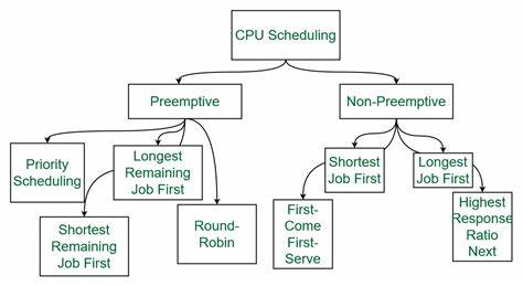
First Come First Serve (FCFS)
This is the simplest CPU scheduling algorithm that schedules according to arrival times of processes. The first come first serve scheduling algorithm states that the process that requests the CPU first is allocated the CPU first. It is implemented by using a FIFO (first-in, first-out) queue. When a process enters the ready queue, its PCB (process control block) is linked to the tail of the queue. When the CPU is free, it is allocated to the process at the head of the queue. The running process is then removed from the queue.
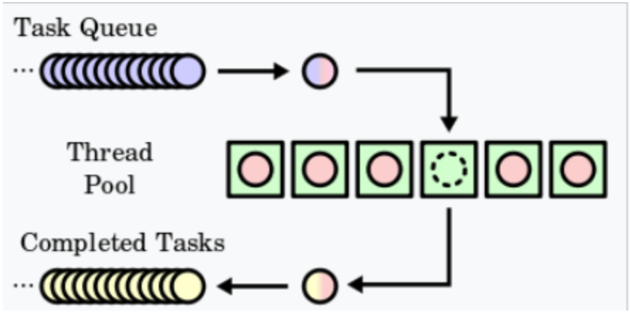
Characteristics of FCFS:
- FCFS supports non-preemptive and preemptive CPU scheduling algorithms.
- Tasks are always executed on a First-come, First-serve concept.
- FCFS is easy to implement and use.
- This algorithm is not very efficient in performance, and the wait time is quite high.
Round Robin Scheduling
Round-robin scheduling allocates each task an equal share of the CPU time. In its simplest form, tasks are in a circular queue and when a task's allocated CPU time expires, the task is put to the end of the queue and the new task is taken from the front of the queue.
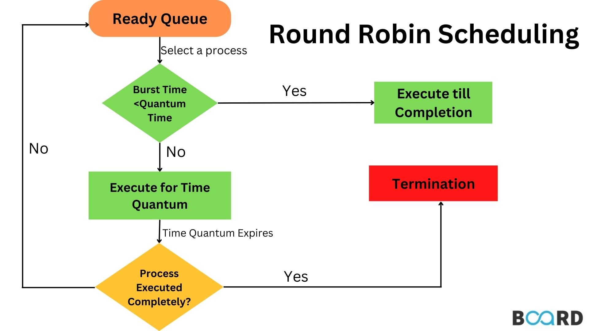
Advantages:
- It is not affected by the convoy effect or the starvation problem as occurred in First Come First Serve CPU Scheduling Algorithm.
Disadvantages:
- Low Operating System slicing times will result in decreased CPU output.
- Round Robin CPU Scheduling approach takes longer to swap contexts.
- Time quantum has a significant impact on its performance.
- The procedures cannot have priorities established.
Shortest Job First Algorithm
In the Shortest Job First (SJF) algorithm, processes are scheduled based on their burst time rather than their arrival time. This algorithm aims to minimize waiting time and maximize throughput. However, a challenge with SJF is that CPU burst times are often not known in advance. To address this, various techniques can be used to estimate burst times, such as analyzing process size or type.

Priority Scheduling
In priority scheduling, each process is assigned a priority number. Depending on the system, a lower or higher priority number indicates higher priority. There are two types of priority scheduling: preemptive and non-preemptive.
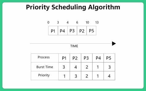
Non-Preemptive Priority Scheduling
In non-preemptive priority scheduling, processes are scheduled based on their priority number. Once a process is scheduled, it runs to completion without interruption. Typically, lower priority numbers indicate higher priority.
Preemptive Priority Scheduling
In preemptive priority scheduling, when a process enters the ready queue, its priority is compared with those of other processes, including the one currently being executed. The process with the highest priority among all available processes is given the CPU. Unlike non-preemptive scheduling, a running process can be interrupted by a higher priority process.
Example
Consider a scenario with 7 processes: P1, P2, P3, P4, P5, P6, and P7. Each process has a priority, arrival time, and burst time. Let's walk through an example to understand how priority scheduling works:
- At time 0, P1 arrives with a burst time of 1 unit and priority 2. Since no other process is available, P1 is scheduled immediately.
- At time 1, P2 arrives. Since P1 has completed execution, P2 is scheduled regardless of its priority.
- At time 2, P3 arrives with a higher priority than P2. Thus, P2's execution is halted, and P3 is scheduled.
- During the execution of P3, three more processes (P4, P5, and P6) become available. However, since their priorities are lower than that of P3, they cannot preempt P3's execution.
- After P3 completes execution, P5, with the highest priority among the remaining processes, is scheduled.
- Once all processes are available in the ready queue, the algorithm behaves as non-preemptive priority scheduling. The process with the highest priority (P4) is executed till completion without interruption.
Challenges
Challenge 1 - Sum and Product Algorithms
This challenge involves implementing the sum and product reductions on an array or memory block of integers. As a bonus challenge, try and make the algorithms more generic and work with any binary operator.
Challenge 2 - Array Concatenation
In this challenge you have to implement an array concatenation function. This should join two arrays of the same type into a single array, similar to strcat(). You will need to allocate a new block of memory and in order to store the concatenated arrays which will requires the sizes of the two input arrays to be known by the function. This function should return a pointer to the resulting array.
Note: The type of the array this function concatenates can be any type except
char.
Challenge 3 - Doing it in Docker
Pull an Ubuntu image from the Docker registry, install any required dependencies and execute the same C code that you wrote for challenge 2 within that running container instance.
Challenge 4 - Bash Process Dump
Write and execute a Bash script that captures the process id, process (cmd) name and Nice score and outputs it all into a text file.
Challenge 5 - Scheduler evaluation
Write a C program that computes the average turnaround time based on these process stats:
| Process | Arrival Time | Burst Time |
|---|---|---|
| P1 | 0 | 3 |
| P2 | 1 | 5 |
| P3 | 2 | 2 |
| P4 | 3 | 4 |
| P5 | 4 | 6 |
M3 & SLURM
M3 is part of MASSIVE, which is a High Performance Computing facility for Australian scientists and researchers. Monash University is a partner of MASSIVE, and provides a majority of the funding for it. M3 is made up of multiple different types of servers, with a total of 5673 cores, 63.2TB of RAM, 5.6PB of storage, and 1.7 million CUDA cores.
M3 utilises the Slurm workload manager, which is a job scheduler that allows users to submit jobs to the cluster. We will learn a bit more about this later on.
This book will introduce the theory behind HPC clusters and how parallel & distributed computing works on these systems. After this, you will learn how to connect to and use M3 along with how SLURM works and how to submit jobs and take advantage of the massive computational capability that M3 provides.
What is HPC really?
You are all likely familiar with the definition of High Performance Computing. Here is one from IBM,
High-performance computing (HPC) is technology that uses clusters of powerful processors that work in parallel to process massive multi-dimensional data sets, also known as big data, and solve complex problems at extremely high speeds. HPC solves some of today’s most complex computing problems in real time.
But the term HPC is not really used much outside the scientific research community. A lot of cloud systems involve similar scale of hardware, parallel & distributed computing, similar computational workload, data processing capacity and low latency/high throughput capability as HPC clusters. So what exactly is the difference between a cloud system and a HPC cluster?
At the end of the day this comes down to semantics but a key difference is that a HPC cluster implies a system primarily used for batch processing whereas a cloud system would involve interactive processing.
Batch Processing vs. Cloud Computing
The vast majority of computer systems and nearly 100% of the ones that the average person uses is a cloud-based interactive system. Due to the nature of use cases specific to researchers, batch processing is a much more suitable choice for them.
Batch Processing:
- Jobs (code scripts) submitted are executed at a later time.
- User can't interact (or only limited interaction).
- Performance measure is throughput.
- Snapshot of output is used for debugging.
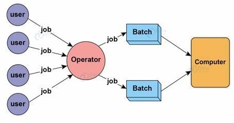
Interactive Processing:
- Jobs submitted are executed immediately.
- User can interact.
- Performance measure is response time.
- Interactive debugging.
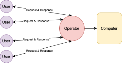
Parallel & Distributed Computing
Nearly all modern computer systems utilise parallel computing to speed up the execution of algorithms. To see how this works in practice look at the diagram below.
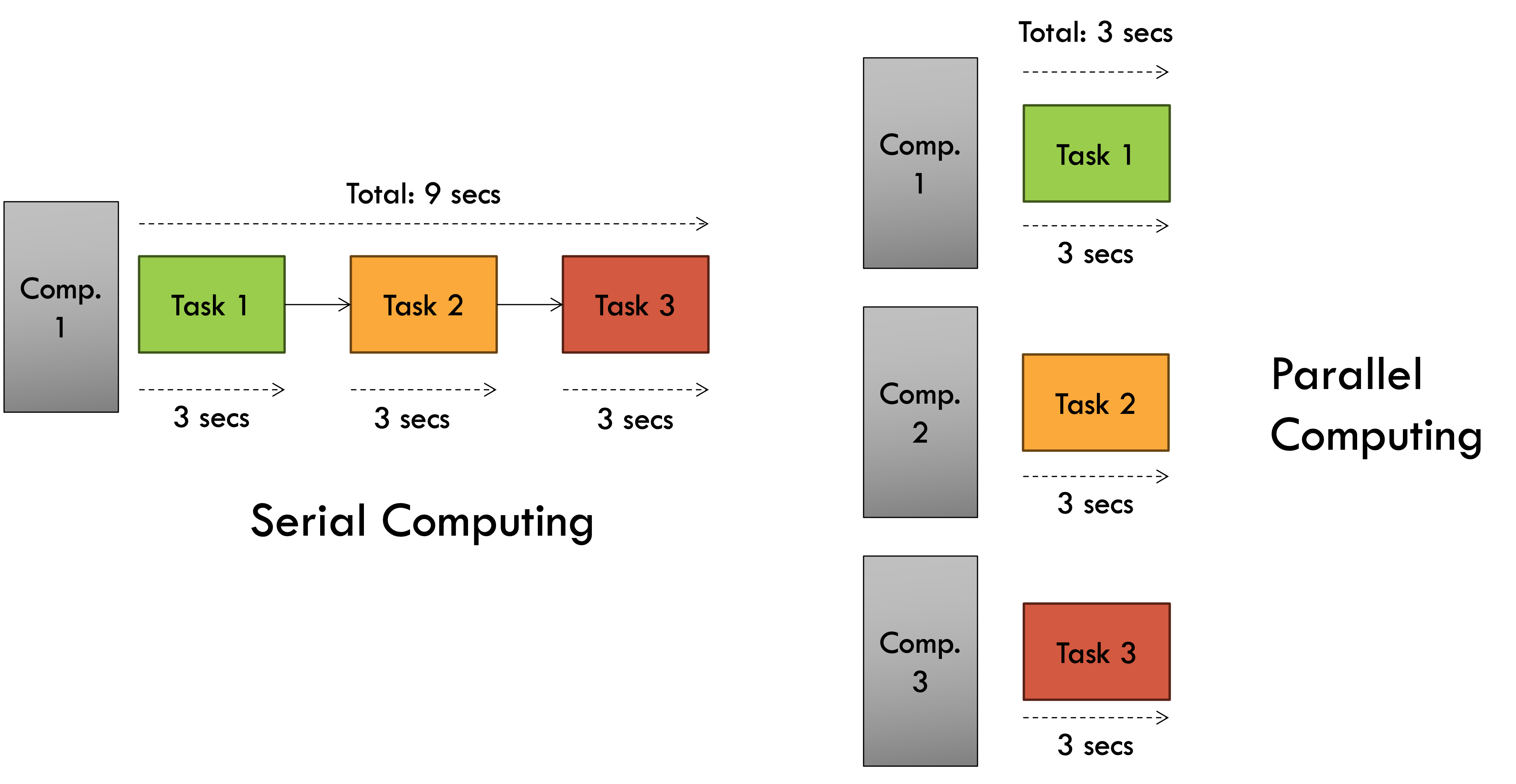
As you can see, in a scenario where a program (job) takes 3 seconds and 3 independent jobs have to be executed by a system, doing it serially in a single processor (computer) takes a total of 9 seconds. But doing it simultaneously across 3 processors will only take 3 seconds thus achieving a 3x speedup through parallel computing. This parallel computing is performed locally in a multi-processing systems with more than 1 CPU core (processor).
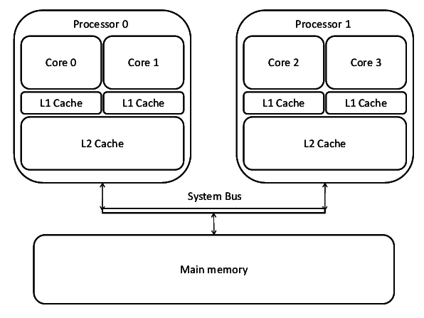
This is the fundamental principle that High Performance Computing is based on. The trouble (or fun) is when your tasks have dependencies on each other which is gonna be the case for the vast majority of algorithms. That's when things like synchronisation issues, data sharing and all of that comes into play - which we'll explore in later chapters.
What is Distributed Computing?
Distributed computing is parallel execution on a distributed memory architecture.
This essentially means it is a form of parallel computing, where the processing power is spread across multiple machines in a network rather than being contained within a single system. In this memory architecture, the problems are broken down into smaller parts, and each machine is assigned to work on a specific part.
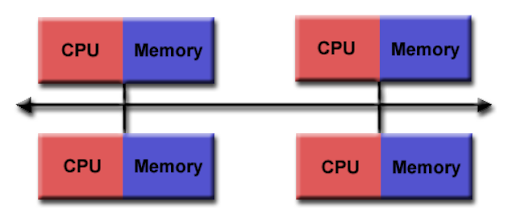
Distributed Memory Architecture
Lets have a look at the distributed memory architecture in more details.
- Each processor has its own local memory, with its own address space
- Data is shared via a communications network using a network protocol, e.g Transmission Control Protocol (TCP), Infiniband etc..
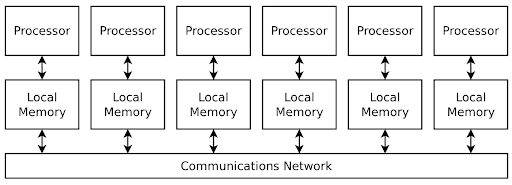
Each machine or node is connected to the HPC cluster via a network, typically one with high bandwidth and low latency. The fact that these are largely independent computers connected over a network rather than a set of CPU/GPU cores in the same computer (in parallel computing), presents a set of disadvantages.
Advantages of parallel & local computing:
- Less data transfer latency than a distributed system. The system bus inside a machine has a much lower latency compared to even the fastest computer networks.
- No need to deal with network congestion related issues and complexities involved in setting up, connecting and managing networks.
- Inter-process communication is a lot simpler on a local computer compared to a distributed system (can just use OpenMP instead of MPI).
On the other hand, there is a reason why most modern computer systems - both cloud & HPC, use distributed computing.
Scaling Up vs Scaling Out
Any time you want to make a computer system more powerful you have two choices - you either scale "up" or you scale "out".
- Scale up: This involves the most intuitive way to increase computational capability. Simply upgrade your system to have more powerful hardware i.e. Increased RAM memory, CPU frequency, no. of cores, etc...
- Scale out: This is where distributed and parallel computing shines. Instead of upgrading the hardware of existing systems, you just add more computers (node) to the system and use distributed computing software to take advantage of the expanded network.
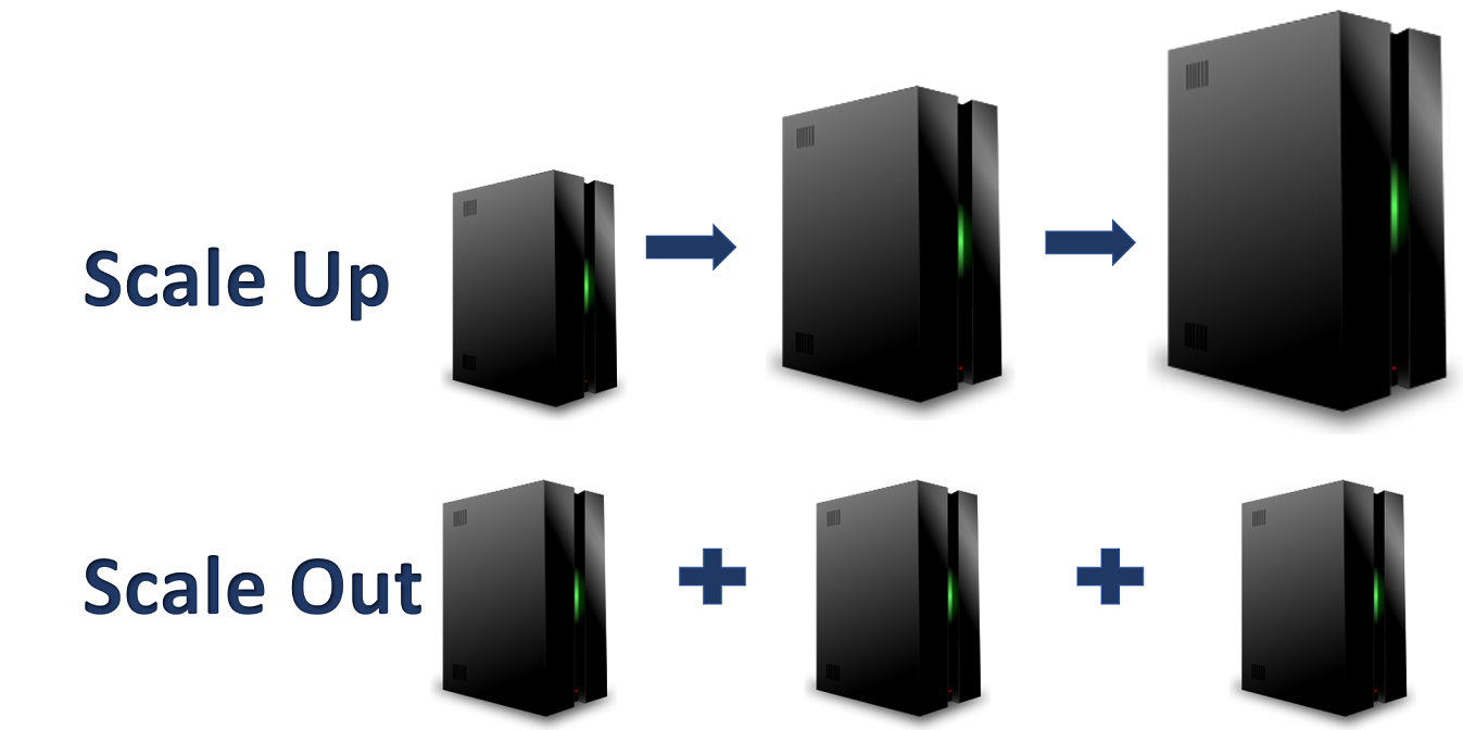
Advantages of distributed computing (scaling out):
- It's usually cheaper and better value for money to add new, cheap computers (nodes) to a HPC cluster than rotate existing computers with upgraded hardware.
- Better redundancy and disaster recovery when you're relying on more than one computer. Adding more nodes to your system allows you to do things like duplicate data and prepare for system meltdowns.
- Fewer I/O bottleneck issues. In a single computer there's only so many additional CPU cores, RAM and secondary storage you can add before the memory addressing system faces bottlenecks. A distributed computing system has nodes with their own individual processors and memory.
And finally, not everything needs to be done on a parallel or distributed system. There are certain issues with this paradigm (explored in more detail in later chapters) that result in certain advantages for serial computing.
Advantages of serial computing:
- More simple to design & implement algorithms. Parallel algorithms can get quite complex, especially when dealing with more complicated instructions with dependencies.
- Less overhead involved in managing a parallel & distributed job. No need to manage data sharing between threads, processes, nodes, etc...
- No synchronisation issues & headaches involved in concurrent computing. Don't have to deal with race conditions, deadlocks, livelocks, etc...
Accessing M3 MASSIVE
The M3 MASSIVE supercomputer has a particular kind of distributed computing architecture called the master-slave architecture. The master (aka driver) node in SLURM & M3 is referred to as the login node while the slave nodes are the compute nodes.
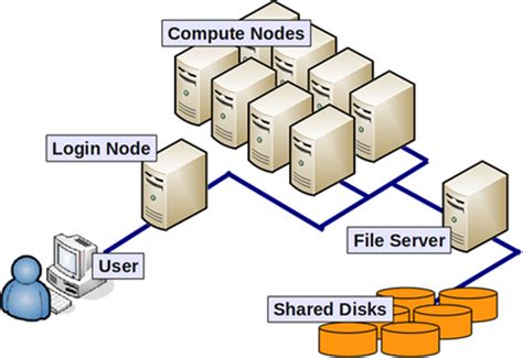
To access the M3 cluster's login node you have two options,
- Use the SSH protocol in a terminal session.
- Use Strudel (webapp built on top of SSH) to create a desktop session.
Login via SSH
Windows
If you are using windows, the best way to ssh into m3 is by using puTTY.
Once installed and opened, you will see a page like this:
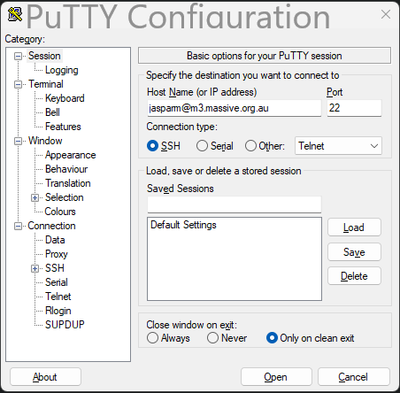
Type in your m3 username followed by @m3.massive.org.au and press enter or the Open button.
If it the first time accessing M3 from this client then you may see something like this:
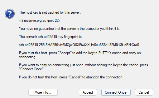
Just click Accept, and puTTY will add the cluster's ssh fingerprint to cache.
Mac / Linux
On macOS or linux, ssh is built into the terminal, so just copy the following into your shell, substituting username for your username.
ssh username@m3.massive.org.au
You may get a similar warning to the above image about the server identity, just type yes or Y to accept it and add the ssh key to cache.
Note: It is possible to use VSCode's built in terminal to ssh into M3, but it is not recommended. It puts unnecessary strain on the login nodes. M3 have a guide on how to correctly connect to M3 using VSCode, however it is quite involved and not particularly necessary unless you want to do proper development on M3 and want to use VSCode to program in.
Everything from now on will be the same across whatever computer you are using to access the cluster.
The first thing to pop up will be a request for a password. Don't worry when you don't see your cursor moving when typing, this is just for security. Your password is still being recorded.
Once you have logged in, you will come to a page that looks like this:
+----------------------------------------------------------------------------+
|                            Welcome to MASSIVE M3                           |
|                                                                            |
|    For assistance please contact help@massive.org.au or (03) 9902 4845     |
|     The MASSIVE User Guide          https://docs.massive.org.au            |
+----------------------------------------------------------------------------+

  - Useful Slurm Commands:
     squeue
     sbatch <slurm_script_file>
     scontrol show job <JOBID>
     scancel <JOBID>

  - Massive User Scripts:
     show_job
     show_job <JOBID>
     show_cluster
     user_info

  - Slurm Sample Scripts are Here:
     /usr/local/hpcusr/latest/training/samples/slurm/

  - We recommend using smux to compile and test code on compute nodes.
  - How to use smux: https://docs.massive.org.au/M3/slurm/interactive-jobs.html

 For more details, please see:
    https://docs.massive.org.au/M3/slurm/slurm-overview.html
------------------------------------------------------------------------------

Use MASSIVE Helpdesk to request assistance with MASSIVE related computing
questions and problems. Email to help@massive.org.au and this will generate
a ticket for your issue.

------------------------------------------------------------------------------


[jasparm@m3-login2 ~]$
Once you are done and want to logout, just type exit. This will close the connection.
Login via Strudel
STRUDEL is a web application used to connect to M3. There are two main benefits to this over regular ssh. Firstly, you are able to access a desktop session, so you can interact easier with M3, look at graphs, etc.. STRUDEL also enables the use of Jupyter notebooks, which are especially useful for data science and machine learning.
Accessing STRUDEL
First, go to the STRUDEL website. You should see something like this:
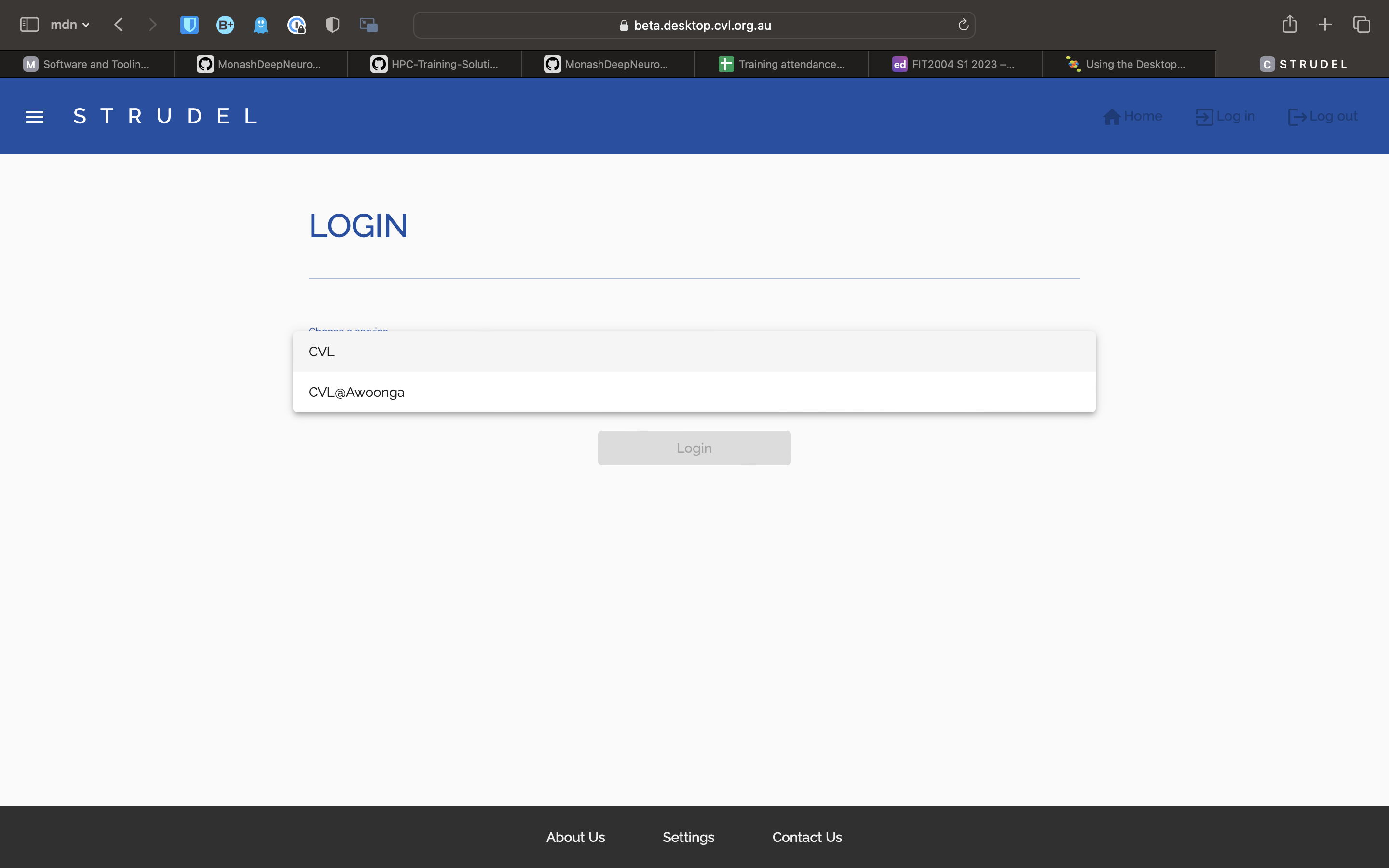
Select the CVL option, and you should be taken to another page, where you choose how to log in.
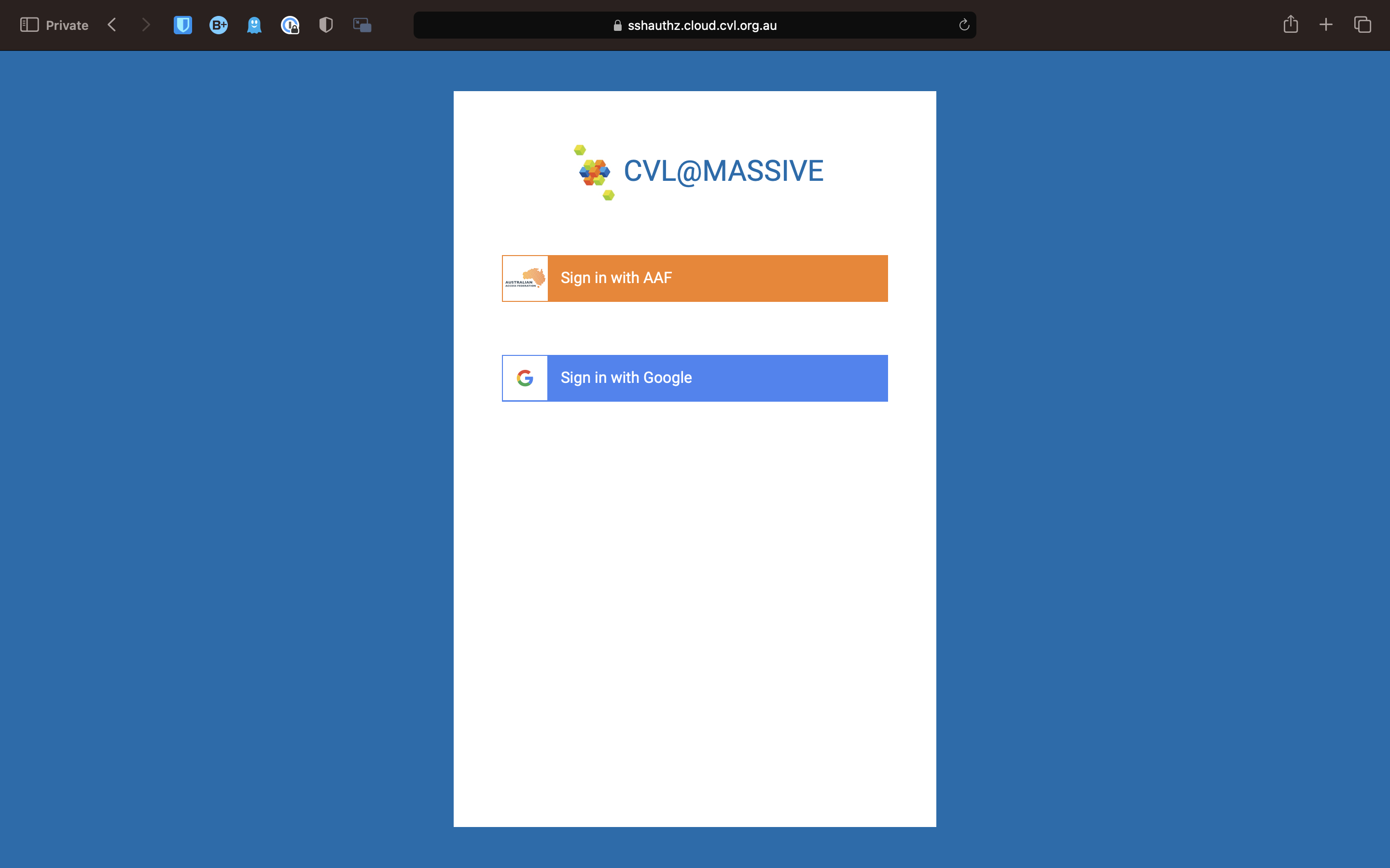
Select AAF. On the next page, search for and select Monash University.
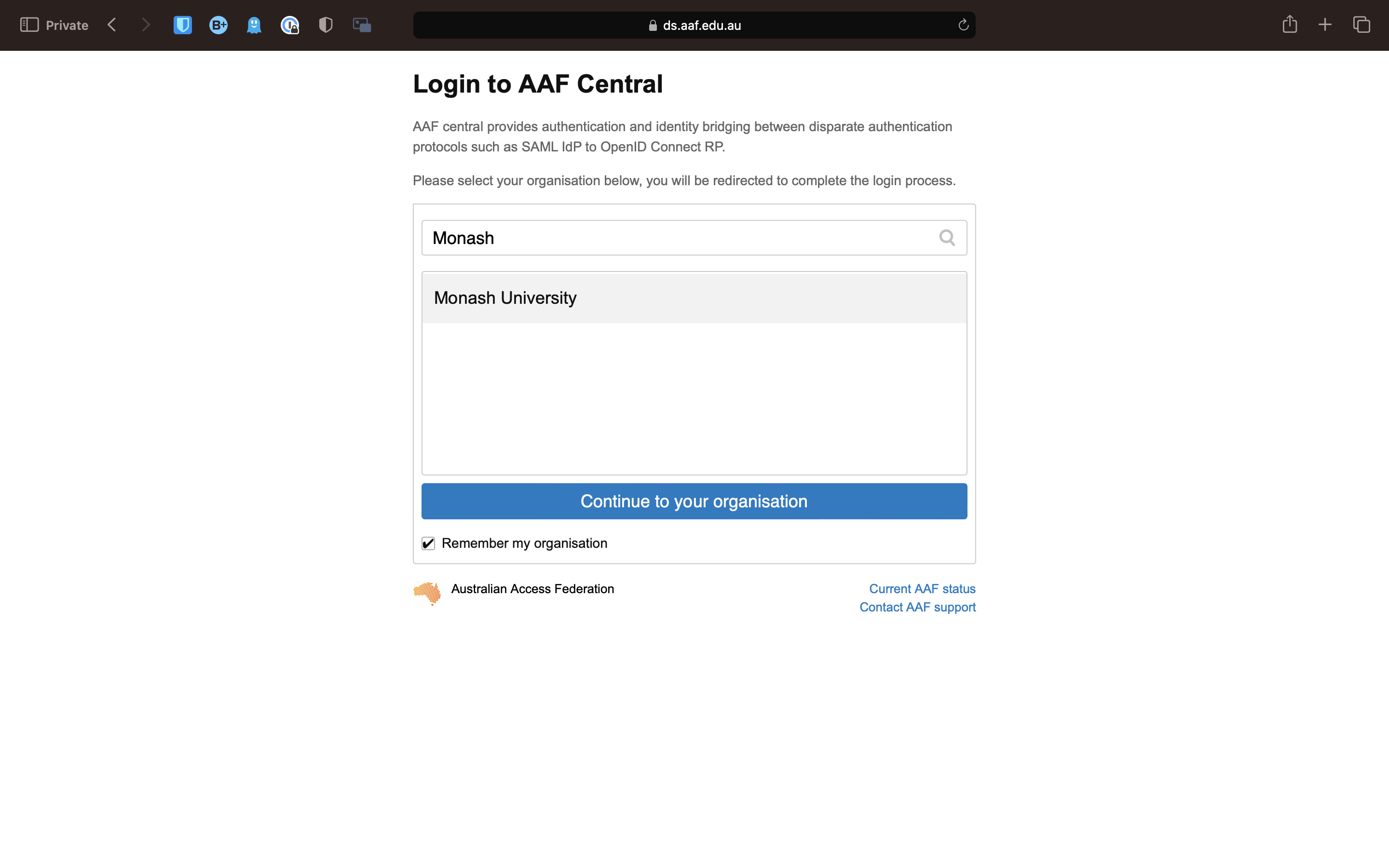
You will now be taken to the Monash login page. Once you have logged in, it will show one last page, asking permission to use your details. Click allow, and you will be taken to the STRUDEL home page.
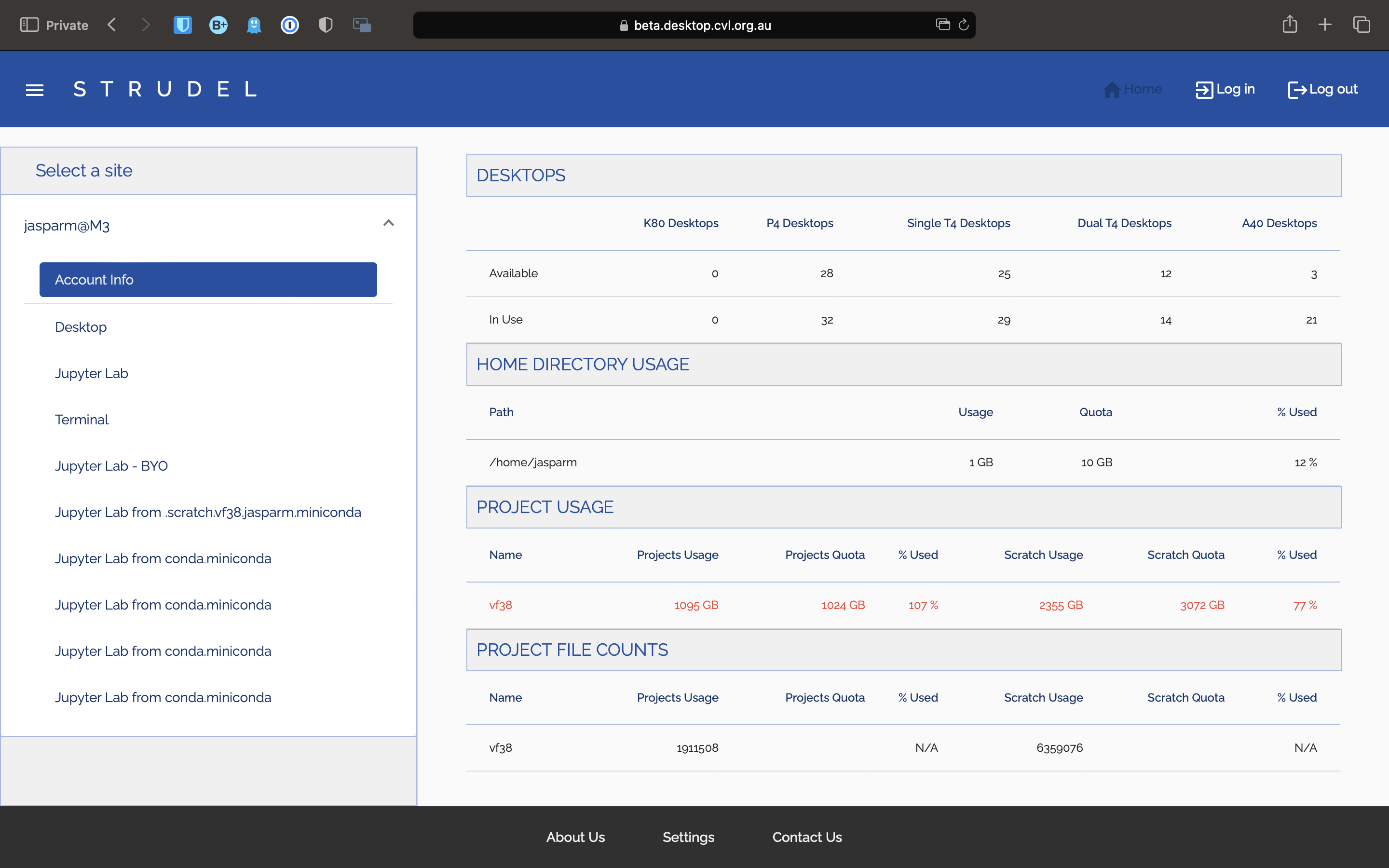
Desktop Session
To start a desktop session using STRUDEL, click on the Desktop tab on the side, select your desired options, and click launch. Once the session has started, you will be able to attach to it by clicking on the connect button in the Pending / Running Desktops section.
Jupyter Notebooks
Similar to Desktops, if you want a basic Jupyter notebook, click on the Jupyter Lab tab, choose how much compute you want, and click launch.
If you want to have a more customised Jupyter notebook, you can do this by first sshing into M3, and activate conda. Then activate the conda environment jupyterlab. Install you desired packages in this environment. Once you have done this, go back to STRUDEL, and launch a Jupyter Lab - BYO session.
SLURM
Slurm (Simple Linux Utility for Resource Management) is an open-source workload manager/scheduler for the M3 MASSIVE cluster. It was created back in the mid-2000s by SchedMd and now it's used by approximately 65% of the world's supercomputers. Slurm is basically the intermediary between the Login node and compute nodes. Hence, the Slurm scheduler is the gateway for the users on the login node to submit work/jobs to the compute nodes for processing.
Slurm has three key functions.
- It provides exclusive and/or non-exclusive access to the resources on the compute nodes to the users for a certain amount of time. Hence, the users can perform any computation with the resources.
- It provides a framework to start, execute, and check the work on the set of allocated compute nodes.
- It manages the queue of pending jobs based on the availability of resources.
The below diagram shows how Slurm works in the context of M3 MASSIVE.
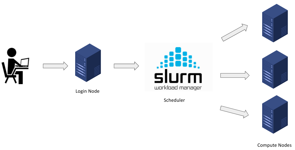
Slurm Architecture
Slurm has a centralized manager, slurmctld, to monitor resources and work. Each compute server (node) has a slurmd daemon, which can be compared to a remote shell: it waits for work, executes that work, returns status, and waits for more work. There is an optional slurmdbd (Slurm DataBase Daemon) which can be used to record job accounting information in a database.
Basic Slurm Commands
Slurm provides a variety of tools for users to submit and manage jobs along with viewing info about them. These commands can be used interactively (on a terminal) in the login node.
| Commands | Syntax | Description |
|---|---|---|
sinfo | sinfo | Get information about the resources on available nodes that make up the HPC cluster. |
sbatch | sbatch <job-id> | Submit a batch script to Slurm for processing. |
srun | srun <resource-parameters> | Run jobs interactively on the cluster. |
skill/scancel | scancel <job-id> | End or cancel a queued job. |
squeue | squeue -u | Show information about your job(s) in the queue. The command when run without the -u flag, shows a list of your job(s) and all other jobs in the queue. |
sacct | sacct | Show information about current and previous jobs. |
Slurm Job Scripting
Slurm job scripts are very similar to bash scripts but you will have to use a set of Slurm-specific directives (flags beginnig #) and Slurm-specific & Bash commands.
In creating a Slurm script, there are 4 main parts that are mandatory in order for your job to be successfully processed.
- Shebang: The Shebang command tells the shell (which interprets the UNIX commands) to interpret and run the Slurm script using the bash (Bourne-again shell) shell.
This line should always be added at the very top of your SBATCH/Slurm script. (Same as all Bash scripts)
- Resource Request: In this section, the amount of resources required for the job to run on the compute nodes are specified. This informs Slurm about the name of the job, output filename, amount of RAM, Nos. of CPUs, nodes, tasks, time, and other parameters to be used for processing the job.
These SBATCH commands are also know as SBATCH directives and must be preceded with a pound sign and should be in an uppercase format as shown below.
#SBATCH --job-name=TestJob
#SBATCH --output=TestJob.out
#SBATCH --time=1-00:10:00
#SBATCH --ntasks=1
#SBATCH --cpus-per-task=1
#SBATCH --mem-per-cpu=500M
Some of the various resource request parameters available for you on Slurm are below:
ntasks: The number of tasks or processes to run.mem: The amount of memory to allocate to the job.time: The maximum amount of time the job can run for.job-name: The name of the job. Up to 15 characters.partition: The partition to run the job on.mail-user: The email address to send job status emails to.mail-type: The types of emails to send.
Note: In the case of M3, a task is essentially the same as a process. This is not the same as a cpu core. You can have a task that uses one or multiple cores. You can also have multiple tasks comprising the same job, each with one or multiple cores being utilised. It can get quite confusing, so if you are unsure about what you need, just ask. There is also more information in the M3 docs.
There are a lot more options that you can use, and you can find a more complete list here.
In particular, if you want to run multithreading or multiprocessing jobs, or you need a gpu, there are more options you need to configure.
- Dependencies: Load all the software that the project depends on to execute. For example, if you are working on a python project, you’d definitely require the python software or module to interpret and run your code. Go to Chapter 5.6 for more info on this.
module load python
- Job Steps Specify the list of tasks to be carried out.
srun echo "Start process"
srun hostname
srun sleep 30
srun echo "End process"
Putting it all together
Please note that the lines with the double pound signs (##) are comments when used in batch scripts.
## Shebang
#!/bin/bash

## Resource Request
#SBATCH --job-name=TestJob
#SBATCH --output=TestJob.out
#SBATCH --time=1-00:10:00
#SBATCH --ntasks=1
#SBATCH --cpus-per-task=1
#SBATCH --mem-per-cpu=500M

## Job Steps
srun echo "`Start process`"
srun hostname
srun sleep 30
srun echo "`End process`"
In the script above, 1 Node with 1 CPU, 500MB of memory per CPU, 10 minutes of Walltime was requested for the tasks (Job steps). Note that all the job steps that begin with the srun command will execute sequentially as one task by one CPU only.
The first job step will run the Linux echo command and output Start process. The next job step(2) will echo the Hostname of the compute node that executed the job. Then, the next job step will execute the Linux sleep command for 30 seconds. The final job step will just echo out End process. Note that these job steps executed sequentially and not in parallel.
It’s important to set a limit on the total run time of the job allocation, this helps the Slurm manager to handle prioritization and queuing efficiently. The above example is a very simple script which takes less than a second. Hence, it’s important to specify the run time limit so that Slurm doesn’t see the job as one that requires a lot of time to execute.
Interactive jobs
Sometimes you might want to actually connect to the node that you are running your job on, in order to see what is happening or to set it up before running the job. You can do this using the smux command. Similar to regular batch jobs, you can set options when you start the interactive session. An example of this is:
smux new-session --ntasks=1 --time=0-00:01:00 --partition=m3i --mem=4GB
This will start an interactive session on a node with 1 cpu, 1 minute of time, and 4GB of memory. There are again other options available, and you can find a more complete explanation here.
Connecting to interactive jobs
Typically when you start an interactive job it will not start immediately. Instead, it will be queued up once it has started you will need to connect to it. You can do this by running smux a, which will reconnect you to the session. If you want to disconnect from the session but leave it running, you can press Ctrl + b followed by d. This will disconnect you from the session, but leave it running. You can reconnect to it later using smux a. If you want to kill the session, if you are connected just run exit, otherwise if you are in a login node run scancel <jobid>. You can find the job id using show_job.
Checking the status of jobs, finding out job IDs, and killing jobs
A couple of useful commands for general housekeeping are:
squeue: This will show you the status of all jobs currently running on M3.show_job: This will show you the status of all jobs you have submitted.squeue -u <username>: This will show you the status of all jobs submitted by a particular user currently running.scancel <jobid>: This will kill a job with a particular job id.scancel -u <username>: This will kill all jobs submitted by a particular user.show_cluster: This will show you the status of the cluster, including any nodes that are offline or in maintenance.
M3 Interface & Usage
Along with Slurm, M3 provides an interface with a set of tools, software packages, commands and a way of working with and using it's directory structure. We provide a brief overview of this interface below. To get more info visit their documentation website.
M3 Specific Commands
| Command | Function |
|---|---|
module load <module_name> | load a module |
module unload <module_name> | unload a module |
module avail | list available modules |
module list | list loaded modules |
module spider <module_name> | search for a module |
module help <module_name> | get help for a module |
module show <module_name> | show details about a module |
module purge | unload all modules |
module swap <module_name> <module_name> | swap two modules |
M3's Shared Filesystem
When we talk about a shared filesystem, what we mean is that the filesystem that M3 uses allows multiple users or systems to access, manage, and share files and directories over a network, concurrently. It enables users to collaborate on projects, share resources, and maintain a unified file structure across different machines and platforms. In addition to this, it enables the many different compute nodes in M3 to access data from a single source which users also have access to, simplifying the process of running jobs on M3.
Very simply, the way it works is that the home, project and scratch directories are mounted on every node in the cluster, so they are accessible from any node.
M3 has a unique filesystem consisting of three main important parts (for you).
Home Directory
There is each user's personal directory, which only they have access to. This has a ~10GB allocation, and should store any hidden files, configuration files, or other files that you don't want to share with others. This is backed up nightly.
Project Directory
This is the shared project directory, for all users in MDN to use. This has a ~1TB allocation, and should be used only for project specific files, scripts, and data. This is also backed up nightly, so in the case that you accidentally delete something important, it can be recovered.
Scratch Directory
This is also shared with all users in MDN, and has more allocation (~3TB). You may use this for personal projects, but keep your usage low. In general it is used for temporary files, larger datasets, and should be used for any files that you don't need to keep for a long time. This is not backed up, so if you delete something, it's gone forever.
General Rules
- Keep data usage to a minimum. If you have a large amount of data, consider moving it to the scratch directory. If it is not necessary to keep it, consider deleting it.
- Keep your home directory clean.
- In general, it is good practice to make a directory in the shared directory for yourself. Name this your username or name, to make it easily identifiable. This is where you should store your files for small projects or personal use.
- The project directory is not for personal use. Do not store files in the project directory that are not related to MDN. Use the scratch directory instead.
Copying files to and from M3
Copying files to and from M3 can be done in a few different ways. We will go over the basics of scp, as well as setting up FileZilla.
A key thing to remember when copying files to and from M3 is that you shouldn't be using the regular ssh url. Instead, they have a dedicated SFTP url to use for file transfers. This is m3-dtn.massive.org.au. This is the url you will use when setting up FileZilla, and when using scp.
Using scp
You can copy files to M3 using the scp command. This is a command line tool that is built into most linux distributions. If you are using Windows, you will need to install a tool like Git Bash to use this command.
Linux / Mac
To copy a file to M3, use the following command:
scp <file> <username>@m3-dtn.massive.org.au:<destination>
For example, if I wanted to copy a file called test.txt to my home directory on M3, I would use the following command:
scp test.txt jasparm@m3-dtn.massive.org.au:~
To copy a file from M3 to your local machine, use the following command:
scp <username>@m3-dtn.massive.org.au:<file> <destination>
So, to bring that same file back to my local machine, I would use the following command:
scp jasparm@m3-dtn.massive.org.au:~/test.txt .
FileZilla
FileZilla is a SFTP client that the M3 staff recommend using. You can download it here.
Once installed, run the program and click on File -> Site Manager or Ctrl-S. This will open the site manager. Click on New Site, and enter the following details:
- Protocol: SFTP
- Host:
m3-dtn.massive.org.au - Logon Type: Ask for password
- User:
<your username>
Don't change anything else. Leave password blank for now.
It should look something like this:
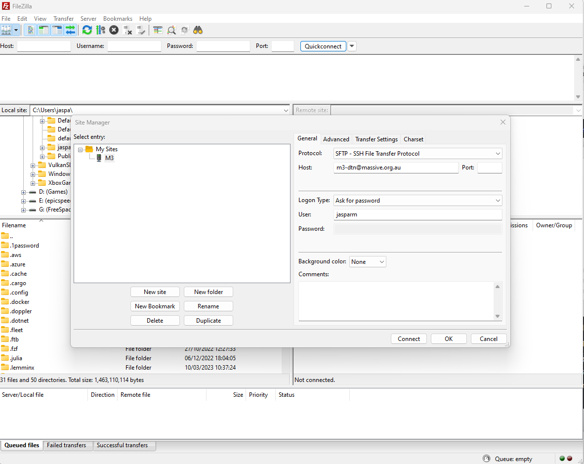 Click on Connect, and enter your password when prompted. You should now be connected to M3. You can now drag and drop files to and from M3.
Software and Tooling
Software and development tooling is handled a little differently on M3 than you might be used to. In particular, because M3 is a shared file system, you do not have access to sudo, and you cannot install software on the system manually. Instead, you will need to use the module command to load software and development tools.
Module
The module command is used kind of as an alternative to package managers like apt or yum, except it is managed by the M3 team. It allows you to load software and development tools into your environment, and is used to load software on M3. To see a comprehensive list of commands go here.
In general, however, you will only really need to use module load and module unload. These commands are used to load and unload software and development tools into your environment.
For most of the more popular software packages, like gcc, there are multiple different versions available. You will need to specify which version you want to load based on your needs.
C
GCC
To load GCC, you can run the following command:
module load gcc/10.2.0
This will load GCC 10.2.0 into your environment, and you can use it to compile C/C++ programs as described in the Intro to C chapter. To unload GCC, you can run the following command:
module unload gcc/10.2.0
Python
Python is a bit of a special case on M3. This is because of how many different versions there are, as well as how many different packages are available. To make things easier, it is recommended that you use miniconda or anaconda to manage your python environments instead of using the system python.
These instructions are based off the M3 docs, which can be found here.
Miniconda
Installing Miniconda
To install Miniconda on M3, there is a dedicated install script that you can use. This will install miniconda into your default scratch space, i.e. /vf38_scratch/<username>/miniconda3. To install miniconda, run the following command:
module load conda-install

# To install miniconda to the default location
conda-install

# To install miniconda to a custom location
conda-install your/install/location
Activating Miniconda
To activate the base conda environment, run the following command:
source your/install/location/miniconda/bin/activate
You will notice that once activated, (base) will appear in the prompt before your username.
To create and activate Python environments within Miniconda, follow these steps:
# Create a new environment
# Change env-name to whatever you want to call your environment
conda create --name env-name python=<version>

# Activate the environment
conda activate env-name
Managing Python packages
Use the following commands to install and manage Python packages:
# Install a package
conda install package-name

# Update a package
conda update package-name

# You can also change the version of packages by adding a = and the version number

# Remove a package
conda remove package-name
Deactivating Miniconda
To deactivate the conda environment you are in, run conda deactivate. To exit conda entirely run conda deactivate again. You will know you have fully exited conda when (base) is no longer in the prompt.
VIM
VIM is a terminal based text editor. You may have heard about it, or even tried using it before. If so, you might recognise the common meme of "how do I exit VIM???". This is because VIM uses a very different key binding system to other text editors, and it can be a little confusing to get used to. However, once you get used to it, it is actually a very powerful and efficient text editor.
I will attemt to give a brief overview of VIM commands, however you should really check out the VIM documentation if you want to learn more.
VIM also has a built in tutorial that you can access by running :help while in VIM.
To use VIM to edit a file, just type vim <filename> into the terminal. This will open the file in VIM. If the file does not exist, it will create a new file with that name.
VIM has three different modes. The first is the command mode, which is the default mode when you open a file. In this mode, you can navigate around the file, and perform other commands. The second is the insert mode, which is used to insert text into the file. The third is the visual mode, which is used to select text.
To enter the insert mode, press i. To exit the insert mode, press esc. To enter the visual mode, press v. To exit the visual mode, press esc.
In command mode, you move around using h, j, k, l. To move along words, press w or b. To move to the start or end of the line, press 0 or $. You can delete a line using dd, or delete a word using dw. You might be noticing some patterns here. In VIM, commands are made up of single or multiple characters that represent different things. For example, if I wanted to delete a word, I would press d to delete, and then w to delete a word. If I wanted to delete 3 words, I would press d3w. If I just wanted to change a word, I would press c instead of d. If I wanted to change 3 words, I would press c3w. If I wanted to change a line, I would press cc. Some other useful command mode commands are u to undo, o to insert a new line and go into insert mode, and ? to search for a string.
To get to insert mode, there are a lots of different ways, but the most common are i to insert text before the cursor, a to insert text after the cursor, and o to insert a new line. The capital versions of these also do things. I inserts text at the start of the line, A inserts text at the end of the line, and O inserts a new line above the current line. To exit insert mode, press esc.
To get to visual mode, press v. In visual mode, you can select text using the same commands as in command mode. To delete the selected text, press d. To change the selected text, press c. To copy the selected text, press y. To paste press p. To exit visual mode, press esc.
To exit VIM itself, enter command mode, and then press :q!. This will exit VIM without saving any changes. To save and exit, press :wq. To save without exiting, press :w.
M3 Challenges
Challenge 1
Navigate to your scratch directory and, using vim (or your chosen in-terminal editor) create a file called hello.txt that contains the text "Hello World". Once you have created the file, use the cat command to print the contents of the file to the screen.
Challenge 2
Write a bash script that prints the contents of the above hello.txt file to the screen and run it locally (on your login node).
Challenge 3
Submit the above script to the queue by writing another SLURM bash script. Check the status of the job using squeue. Once the job has finished, check the output using cat. You can find the output file in the directory you submitted the job from.
Challenge 4
Request an interactive node and attach to it. Once you have done this, install python 3.7 using conda.
Challenge 5
Clone and run this script. You will need to first install the dependencies for it. You don't need to wait for it to finish, just make sure it is working. You will know its working if it starts listing out the loss and accuracy for each epoch. You can stop it by pressing ctrl + c.
Once you have confirmed that it is working, deactivate and delete the conda environment, and then end the interactive session.
Hint: I have included the dependencies and their versions (make sure you install the right version) in the
requirements.txtfile. You will need python 3.7 to run this script.
Challenge 6
Go back to the login node. Now you are going to put it all together. Write a bash script that does the following:
- (1) requests a compute node
- (2) installs python using conda
- (3) clones and runs the above script
Let this run fully. Check the output of the script to make sure it ran correctly. Does it match the output of the script you ran in challenge 5?
Hint: You can check the output of the script at any time by
cating the output file. The script does not need to have finished running for you to do this.
Challenge 7
Edit your submission script so that you get a gpu node, and run the script using the gpu.
Hint: Use the m3g partition
Challenge 8
Now you want to clean up your working directory. First, push your solutions to your challenges repo. Then, delete the challenges directory, as well as the conda environment you created in challenge 6.
Parallel Computing
As introduced in chapter 5, parallel computing is all about running instructions simultaneously on multiple computers rather than doing it all sequentially/serially on the same computer. This is relatively straightforward if we have multiple, completely independent tasks that don't need to share resources or data i.e. inter-query parallelism.
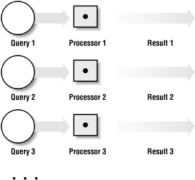
In this context, you can consider a query to be a job that carries out a series of steps on a particular input in order to achieve something e.g. a SORT query on a table. It's fairly straightforward to execute multiple queries at the same time using a parallel/distributed system but what if we want to parallelise and speed up the individual operations within a query?
This is where things like synchronisation, data/workload distribution and aggregation needs to be considered. In this chapter we will provide some theoretical context before learning how to implement parallelism using OpenMP & MPI.
Parallel Algorithms
You can think of all parallel algorithms as having a serial portion and a parallel portion i.e. local and global phases.
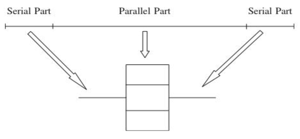
This applies to both local parallel computing between CPU cores with a shared RAM as well as distributed computing between multiple HPC nodes with a distributed memory architecture. The only difference between the two is additional complexities involved in managing data sharing & sending instructions across a network.
Let's go through this with a simple example. To calculate the sum of all numbers between 1 to N serially, you would execute the following pseudocode,
function sumOfNumbers(N):
    result = 0

    for x from 1 to N:
        result += x

    return result
To do this in parallel (assuming you have M processors/nodes) you would do something like this,
function parallelSum(N):
    globalResult = 0
    partition_size = N // M

    for node from 1 to M:
        partition = node * partition_size
        localResult = sendJobToNode(node, sumOfNumbers(partition))
        globalResult += localResult

    return globalResult
This is how one of the simplest parallel algorithms - parallel sum works. All lines of code beside the sendJobToNode function call are executed serially on the master node/thread. This is all illustrated in the diagram below.
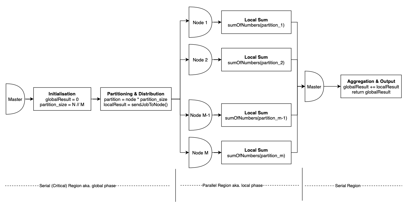
Besides the difference between serial & parallel regions another important concept to note here is partitioning aka. chunking. Often when you're parallelising your serial algorithm you will have to define local, parallel tasks that will execute on different parts of your input simultaneously in order to acheive a speedup. This can be anything from a sum operation in this case, to a local/serial sort or even as complex as the training of a CNN model on a particular batch of images.
Multithreading
Hopefully by now you are all familiar with multi-threading and how parallel computing works. We'll now go through how to implement parallel computing using OpenMP in order to speed up the execution of our C programs.
OpenMP
OpenMP is an Application Program Interface (API) that is used to implement multi-threaded, shared memory parallelism in C/C++ programs. It's designed to be a very minimal add-on to serial C code when it comes to implementation. All you have to do is use the #pragma (C preprocessor directives) mechanism to wrap the parallel regions of your code.
Fork-Join Parallel Execution Model
OpenMP uses the fork-join model of parallel execution.
- FORK: All OpenMP programs begin with a single master thread which executes sequentially until a parallel region is encountered. After that, it spawns a team of threads to carry out the multi-threaded parallel computing.
The OpenMP runtime library maintains a pool of potential OS threads that can be added to the thread team during parallel region execution. When a thread encounters a parallel construct (pragma directive) and needs to create a team of more than one thread, the thread will check the pool and grab idle threads from the pool, making them part of the team.
This speeds up the process of thread spawning by using a warm start mechanism to minimise overhead associated with the kernel scheduler context switching needed to conduct thread spawning.
If you're unclear how the kernel scheduler context switching works, revisit the operating systems chapter and explore/lookup the topics introduced there.
- JOIN: Once the team of threads complete the parallel region, they synchronise and return to the pool, leaving only the master thread that executes sequentially.
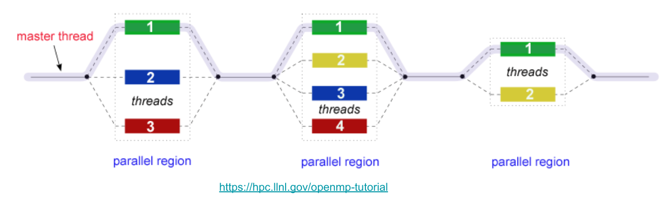
Imperative vs Declarative
Imperative programming specifies and directs the control flow of the program. On the other hand, declarative programming specifies the expected result and core logic without directing the program's control flow i.e. you tell the computer what to do instead of how to do it.
OpenMP follows a declarative programming style. Instead of manually creating, managing, synchronizing, and terminating threads, we can achieve the desired outcome by simply declaring pragma directives in our code.
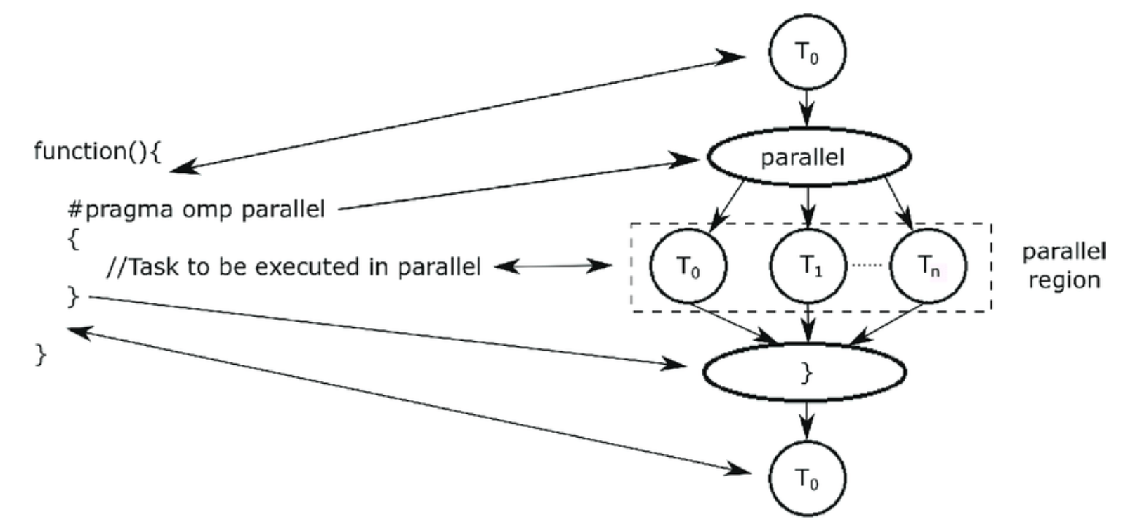
Working with OpenMP
We will now look at a simple example.
The code can be compiled with
gcc -fopenmp -o hello hello.c.
#include <omp.h>
#include <stdio.h>

int main() {
    int i;
    #pragma omp parallel for
    for (i = 0; i < 10; i++) {
        printf("Thread %d executing iteration %d\n", omp_get_thread_num(), i);
    }
    return 0;
}
Running on M3
Here is a template script provided in the home directory in M3. Notice that we can dynamically change the number of threads using export OMP_NUM_THREADS=12.
The
exportstatement is a bash command you can type into a WSL/Linux terminal. It allows you to set environment variables in order to manage runtime configuration.
#!/bin/bash
# Usage: sbatch slurm-openmp-job-script
# Prepared By: Kai Xi,  Apr 2015
# NOTE: To activate a SLURM option, remove the whitespace between the '#' and 'SBATCH'

# To give your job a name, replace "MyJob" with an appropriate name
# SBATCH --job-name=MyJob

# To set a project account for credit charging,
# SBATCH --account=pmosp

# Request CPU resource for a openmp job, suppose it is a 12-thread job
# SBATCH --ntasks=1
# SBATCH --ntasks-per-node=1
# SBATCH --cpus-per-task=12

# Memory usage (MB)
# SBATCH --mem-per-cpu=4000

# Set your minimum acceptable walltime, format: day-hours:minutes:seconds
# SBATCH --time=0-06:00:00

# To receive an email when job completes or fails
# SBATCH --mail-user=<You Email Address>
# SBATCH --mail-type=END
# SBATCH --mail-type=FAIL

# Set the file for output (stdout)
# SBATCH --output=MyJob-%j.out

# Set the file for error log (stderr)
# SBATCH --error=MyJob-%j.err

# Use reserved node to run job when a node reservation is made for you already
# SBATCH --reservation=reservation_name

# Command to run a openmp job
# Set OMP_NUM_THREADS to the same value as: --cpus-per-task=12
export OMP_NUM_THREADS=12
./your_openmp_program
Synchronisation
Synchronisation is the task of coordinating multiple processes (or threads) to join up or handshake at a certain point, in order to reach an agreement or commit to a certain sequence of action. This is important so that the different threads/processes you spawn in the parallel region don't contradict each other and corrupt your code.
Race Condition
A race condition is one of the most popular forms of this synchronisation corruption. It's essentially when your threads are in a "race" against each other to access a particular resource (eg. an int variable's value) and the loser's access/update to that resource is lost.
Instead of your threads fighting each other, you want them to work together perfectly synchronised i.e. more like an F1 pitstop crew than a toxic office place.
Let's start with this simple program:
/*
We purposefully added the following code within the program:
- The sleep() calls allow thread switching in the middle of function calls.
- The silly variable assignments in increment() mimic the register.
- All functions are sharing a global counter variable.

Note that:
- Even if we remove all of the sleep() and the variable assignments,
the error can still occur by chance.

What should be the desired output?
What is the actual output?
*/
#include <omp.h>
#include <stdio.h>
#include <unistd.h>

float sleep_time = 0.1;
int counter = 0;                                    // Sharing across the program

int get_value() {
    sleep(sleep_time);                              // This will cause thread switching
    printf("Current Counter = %d\n", counter);
    return counter;
}

void increment() {
    int temp = counter;                             // Load counter to register
    sleep(sleep_time);                              // This will cause thread switching
    temp++;                                         // Increment the register
    counter = temp;                                 // Store back to the variable

    printf("Incremented counter to %d\n", counter);
}

int main() {
#pragma omp parallel for
    for (int i = 0; i < 5; i++) {
        increment();
        get_value();
    }

    return 0;
}
Single Thread
Running the program using 1 thread:
export OMP_NUM_THREADS=1
./counter
The output should look something like this:
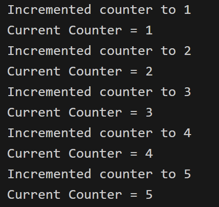
The program works great. No corruption at all.
- This is because we only used 1 single thread.
- The program is just a serial program without any parallelism.
sleep()calls simply put the thread to sleep, that same thread will go to sleep, wake up, and continue the execution.
Multiple Threads
export OMP_NUM_THREADS=2
./counter
Running the program using 2 threads may give us this output:
Note: This is just one possible output.
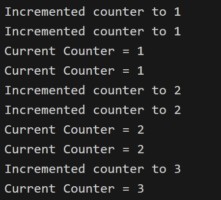
What is happening here?
- We are using 2 threads.
- Both threads are trying to access the global variable
counterat the same time (roughly). - During the time when 1 thread is sleeping, the other thread may increment the shared counter.
- The 2 threads simply go on their way and not coordinate with each other.
This is what a Race Condition is. A race condition occurs when two or more threads can access shared data and they try to change it at the same time.
How to prevent race conditions in OpenMP?
There are a few approaches we can take:
- Critical construct: This restricts the code so that only one thread can do something at a time (in our example, only 1 thread can increment the counter at a time). It's used to specify a critical region which is another term for serial execution.
int main() {
#pragma omp parallel for
    for (int i = 0; i < 5; i++) {
#pragma omp critical                                // Critical construct
        increment();
        get_value();
    }
    return 0;
}
This is unfortunatley not appropriate for some situations since it is bad for performance and destroys a lot of the speed-up we're trying to acheive in the first place.
- Atomic construct: This is quite similar to the critical construct, however it only applies to memory read/write operations. It has a better performance than the critical construct by taking advantage of the hardware. There's no lock/unlock needed on entering/exiting the line of code, it just does the atomic operation which the hardware tells you can't be interfered with. Let's look at another example:
Run this program multiple times using multiple threads (before uncommenting the construct). Again, race condition!
#include <omp.h>
#include <stdio.h>

int total = 0;
int n = 100;
int nums[100];

int main() {
    // Populate nums
    for (int i = 0; i < n; i++) {
        nums[i] = i;
    }

#pragma omp parallel for
    for (int i = 0; i < n; i++) {
        int temp = nums[i];
        /*
        We can easily resolve the race condition with atomic/critical construct.
        The atomic one will work perfectly and give better performance this time.
        Uncomment the construct below to resolve the race condition.
        */
// #pragma omp atomic
        total += temp;
    }
    printf("%d\n", total);
}
- Reduction: Based on the problem, sometimes, the best solution will be to use
reduction. Let's analyse what this code is doing:
Using
reductionhere results in significantly better performance.
- A quick way to do some simple benchmarking is:
time a-command- Conduct benchmarking for 3 versions, and trying in different number of threads
Example:
# Tuning the number of threads
export OMP_NUM_THREADS=4

# Change according to your file's name
time ./critical
time ./atomic
time ./reduction
#include <omp.h>
#include <stdio.h>

int total = 0;
int n = 100;
int nums[100];

int main() {
    // Populate nums
    for (int i = 0; i < n; i++) {
        nums[i] = i;
    }

#pragma omp parallel for reduction(+:total) num_threads(3)
    for (int i = 0; i < n; i++) {
        int temp = nums[i];
        total += temp;
    }
    printf("Final total is: %d\n", total);
}
Notice that:
- The previous two approaches only allow 1 thread at a time to perform some operations.
- Reduction allows threads to access the same shared data at the same time, but in different parts of the data.
The nature of the word synchronisation in these two examples is completely different from each other, while still adhering to our initial definition!
Barrier Synchronisation
In the last sub-chapter, we have talked about the Fork - Join Model. We know that "Once the team of threads complete the parallel region, they synchronise and return to the pool, leaving only the master thread that executes serially.". However, there are a few important aspects that we have left out:
- The time taken to finish the assigned task is different for each thread.
- How can OpenMP know/identify when a thread has completed its own task.
- How can OpenMP know/identify when all threads have finished all the tasks.
The answer lies in something called Barrier Synchronisation. Here are illustrations for the idea:
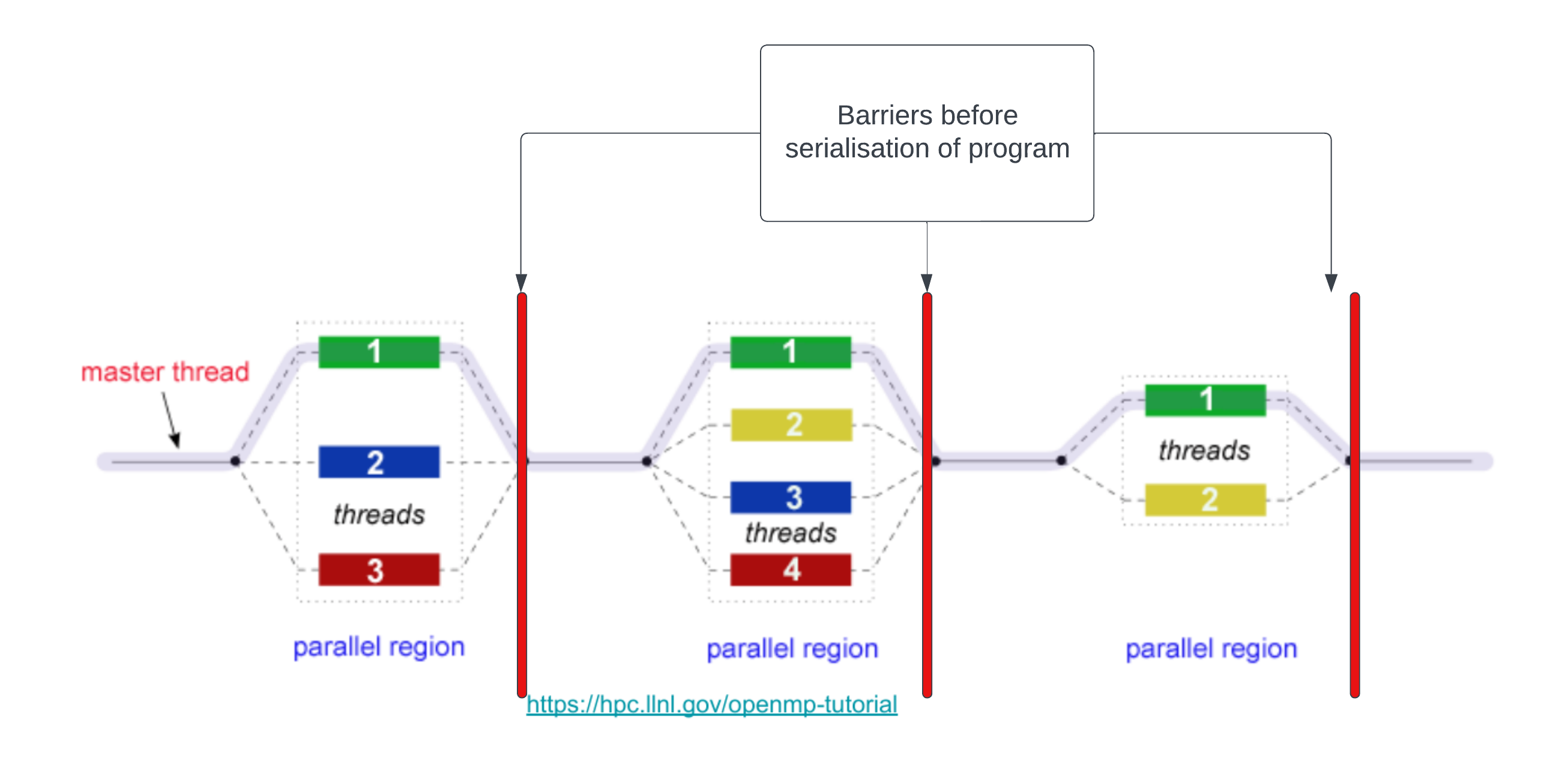
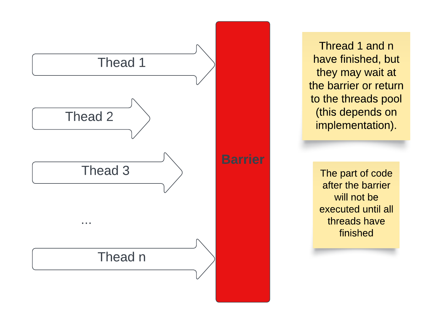
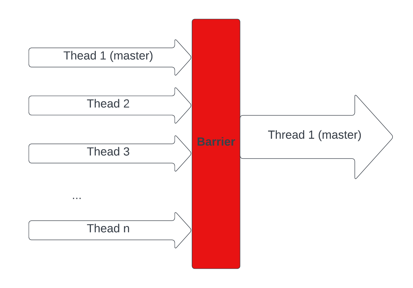
Implicit Barriers
The barrier synchronisation implicitly (behind the scenes) occur at the end of constructs (regions of code) such as parallel constructs ("#pragma omp parallel") and the end of worksharing constructs(loop, sections, single, and workshare constructs).
#include <stdio.h>
#include <omp.h>

int main(void)
{
    #pragma omp parallel {
        // Parallel code
        printf("Thread %d is executing...\n", omp_get_thread_num());
    }

    // Sequential code after the barrier
    printf("Main thread\n");
    return 0;
}
Barrier Construct
The barrier construct specifies an explicit (We add the construct into the code by ourselves) barrier at the point at which the construct appears. The barrier construct is a stand-alone directive. Here is an illustration of the following code.
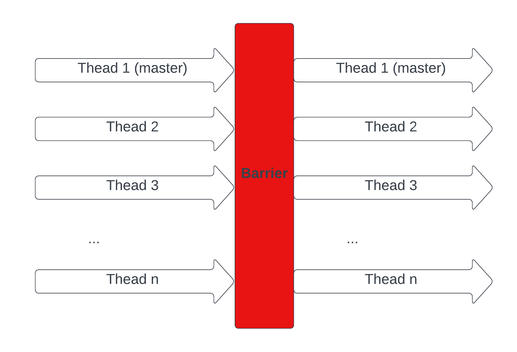
#include <stdio.h>
#include <omp.h>

int main(void)
{
    #pragma omp parallel
    {
        printf("Thread %d executes part 1\n", omp_get_thread_num());
        #pragma omp barrier

        // No thread will execute part 2 before part 1
        printf("Thread %d executes part 2\n", omp_get_thread_num());
    }
    return 0;
}
Let's think about a way to implement a barrier
We don't need to know exactly how OpenMP implemented this feature, at least not right now (if you are interested in OpenMP implementation, here could be a start). We can follow a rough simple approach:
- Let's assume we have
nthreads. - We need a way to count how many threads that have finished, this can easily be done with a shared counter variable (be careful with race condition) among threads. When this counter reaches the number
n, we will know that all threads have finished. - We also need a mechanism to make a finished thread idle and wait() for other threads to finish.
- The last thread to finish has the responsibility of notify() other threads (threads that you want to be executed after the barrier).
Voila! we have a barrier.
Locks
Ealier, we have learnt about how to write concurrent programs, as well as a few constructs to achieve synchronisation in OpenMP. We know that:
reduction constructpartitions shared data and used a barrier to achieve synchronisationatomic constructutilises hardware ability to achieve thread-safe small memory read/write operations.
What about critical construct? We said that it uses locks, but what are locks?
Notes that the direct use of locks is not recommended (at least in OpenMP):
- It is very easy to cause a deadlock or hard-to-debug livelock (more on these at the end of this sub-chapter).
- It can often cause very poor performance or worse.
- It generally indicates that the program design is wrong.
We will explore them because it is important to know about what is happening under the hood of the high-level APIs.
Overall Idea
Lock is a synchronization technique. A lock is an abstraction that allows at most one thread to own it at a time. To be more concrete, let's say we have a segment of code, guarded by a lock. Then, exactly 1 thread can execute those lines of code at a time (Sounds familiar?). Any other threads (without the lock) trying to access the code segment will have to wait until the lock is released.
OpenMP Locks
Let's start with an example:
#include <omp.h>
#include <stdio.h>

int total = 0;
int n = 100;
int nums[100];
omp_lock_t lock;                        // uninitialized

int main() {

    omp_init_lock(&lock);               // the lock is initialized but unlocked

    // Populate nums
    for (int i = 0; i < n; i++) {
        nums[i] = i;
    }

#pragma omp parallel for
    for (int i = 0; i < n; i++) {
        int temp = nums[i];

        omp_set_lock(&lock);            // a thread changes the lock's state to locked

        total += temp;                  // something that we want only 1 thread execute at a time

        omp_unset_lock(&lock);          // the thread owning the lock changes the lock's state to unlocked
    }
    omp_destroy_lock(&lock);
    printf("%d\n", total);
}
An OpenMP lock can exist in three states: uninitialized, unlocked, or locked. When in the unlocked state, a task can acquire the lock, transitioning it to the locked state. The task acquiring the lock is considered its owner. An owning task can release the lock, reverting it to the unlocked state. Any attempt by a task to release a lock it does not own renders the program non-conforming.
There are two types of locks supported: simple locks and nested locks:
- Nested locks allow for multiple acquisitions before unlocking. They remain locked until unset as many times as
omp_set_nest_lockhas been called. Nested locks facilitate scenarios where functions call other functions utilizing the same lock. - Simple locks should be acquired only once using
omp_set_lockand released with a single call toomp_unset_lock.
Deadlocks
When used correctly and cautiously, locks can effectively prevent race conditions. However, there's another issue to be aware of. Because using locks means that threads have to wait (blocking when another thread holds the lock), there's a risk of a situation where two threads end up waiting for each other, leading to a stalemate where neither can progress.
Let's look at this code:
#include <stdio.h>
#include <omp.h>

omp_lock_t lock1, lock2;

int main() {
    omp_init_lock(&lock1);
    omp_init_lock(&lock2);

#pragma omp parallel num_threads(2)
    {
        int thread_id = omp_get_thread_num();

        if (thread_id == 0) {
            omp_set_lock(&lock1);                               // Thread 0 takes lock 1
            printf("Thread %d acquired lock1\n", thread_id);
            omp_set_lock(&lock2);                               // Attemp to take lock 2 (but already belongs to thread 1 => wait)
            printf("Thread %d acquired lock2\n", thread_id);
            omp_unset_lock(&lock2);
            omp_unset_lock(&lock1);
        }
        else {
            omp_set_lock(&lock2);                               // Thread 1 takes lock 2
            printf("Thread %d acquired lock2\n", thread_id);
            omp_set_lock(&lock1);                               // Attemp to take lock 1 (but already belings to thread 0 => wait)
            printf("Thread %d acquired lock1\n", thread_id);
            omp_unset_lock(&lock1);
            omp_unset_lock(&lock2);
        }
    }

    omp_destroy_lock(&lock1);
    omp_destroy_lock(&lock2);

    return 0;
}
The output should be something like this:
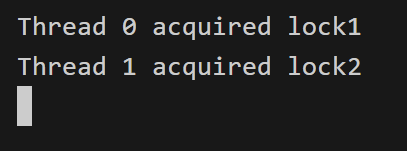
The program is not terminated. However, no thread is making any progress as they are being blocked by each other at the same time!
Deadlock is not just limited to two modules; the key characteristic of deadlock is a cycle of dependencies:
- A is waiting for B
- B is waiting for C
- C is waiting for A
In such a loop, none of the threads can move forward.
Livelocks
A more challenging issue that may arise is livelock. Similar to deadlock, livelocked threads are unable to make progress. However, unlike deadlock, where threads are blocked, livelocked threads remain active. They're caught in a continuous and infinite sequence of responding to each other, preventing them from making any meaningful progress in their work.
#include <stdio.h>
#include <omp.h>
#include <unistd.h>

omp_lock_t lock1, lock2;

void execute_task(int task_number) {
    omp_lock_t* first_lock;
    omp_lock_t* second_lock;
    const char* lock1_message;
    const char* lock2_message;

    if (task_number == 1) {
        first_lock = &lock1;
        second_lock = &lock2;
        lock1_message = "lock1";
        lock2_message = "lock2";
    }
    else {
        first_lock = &lock2;
        second_lock = &lock1;
        lock1_message = "lock2";
        lock2_message = "lock1";
    }

    while (1) {
        omp_set_lock(first_lock);
        printf("%s acquired, trying to acquire %s.\n", lock1_message, lock2_message);

        // sleep for 50 milliseconds to illustrate some meaningful tasks,
        // and to ensures that the order of lock and unlock can not correct itself by chance
        usleep(50000);

        if (omp_test_lock(second_lock)) {
            printf("%s acquired.\n", lock2_message);
        }
        else {
            printf("cannot acquire %s, releasing %s.\n", lock2_message, lock1_message);
            omp_unset_lock(first_lock);
            continue;
        }

        printf("executing task %d.\n", task_number);
        break;
    }
    omp_unset_lock(second_lock);
    omp_unset_lock(first_lock);
}

int main() {
    omp_init_lock(&lock1);
    omp_init_lock(&lock2);

// each section will be executed in parallel
#pragma omp parallel sections
    {
#pragma omp section
        {
            execute_task(1);
        }

#pragma omp section
        {
            execute_task(2);
        }
    }

    omp_destroy_lock(&lock1);
    omp_destroy_lock(&lock2);

    return 0;
}
Message Passing
As each processor has its own local memory with its own address space in distributed computing, we need a way to implement communication between the distributed processes and allow data sharing. Message passing is the mechanism of exchanging data between processes. Each process can communicate with one or more other processes by sending messages over a network.
The MPI (message passing interface) in OpenMPI is a communication protocol standard defining message passing between processors in distributed environments. The main goals of this protocol standard is high performance, scalability, and portability.
OpenMPI is one implementation of the MPI standard. It consists of a set of headers library functions that you call from your program. i.e. C, C++, Fortran etc.
For C, you will need a header file for all the functions mpi.h and link in the relevant library functions. This is all handled by the mpicc program (or your compiler if you wanted to specify all the paths).
OpenMPI
Primary MPI Routines
int MPI_Init(int * argc, char ** argv);
// initializes the MPI environment.
// Argc argv are the parameters come
// from main(argc,argv). The return value is an
// error code. 0 is OK. Non-zero is an error code
int MPI_Comm_size(MPI_Comm comm, int \* size);
// this functions gets the number of MPI processes
// i.e. the number you enter when you go mpirun -np \<size> myprog.exe
// *size is C syntax indicating that size will be modified to contain
// the value after the function returns. The return value is only used
// for error detection. printf(“MPI size is %d\n”,size);
int MPI_Comm_rank(MPI_Comm comm, int \* rank);
// this returns the rank of this particular process
// rank contains the value for that process- the function return value is an error code
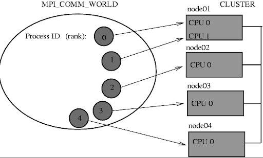
Point-to-Point communication
These are blocking functions - they wait until the message is sent or received. Note that the CPU is actively polling the network interface when waiting for a message. This is opposite in behaviour to other C functions, i.e. c= getChar() (which causes a context switch and then a sleep in the OS). This is done for speed reasons.
int MPI_Send(void * buf, int count, MPI_Datatype type, int dest, int tag, MPI_Comm comm);
Sends a message from the calling process to another process
INPUT PARAMETERS
buf- Initial address of send buffer (choice).
count- Number of elements sent (non negative integer).
type- DataType of each send buffer element (handle).
dest- Rank of destination (integer).
tag- Message tag (integer).
comm- Communicator (handle).
OUTPUT PARAMETER
IERROR- Fortran only: Error status (integer).
int MPI_Recv(void * buf, int count, MPI_Datatype type, int source, int tag, MPI_Comm comm, MPI_Status * status);
Receives a message from another process
INPUT PARAMETERS
count- Maximum number of elements to receive (integer).
type- DataType of each receive buffer entry (handle).
source- Rank of source (integer).
tag- Message tag (integer).
comm- Communicator (handle).
OUTPUT PARAMETERS
buf- Initial address of receive buffer (choice).
status- Status object (status).
IERROR- Fortran only: Error status (integer).
Primary MPI Routines closing
In a header file you will find
int MPI_Finalize(void);
To call in your C or C++ program
#include <mpi.h>
MPI_Finalize();
General overview MPI program
...
int MPI_Init(int  argc, char ** argv);
--------------------------Parallel algorithm starts----------------------
int MPI_Comm_size(MPI_Comm comm, int * size);
int MPI_Comm_rank(MPI_Comm comm, int * rank);
...
int MPI_Send(void * buf, int count, MPI_Datatype type, int dest, int tag, MPI_Comm comm);
int MPI_Recv(void * buf, int count, MPI_Datatype type, int source, int tag, MPI_Comm comm, MPI_Status * status);
…
--------------------------Parallel algorithm ends-----------------------
int MPI_Finalize(void);
...
Terminology:
- World Size: The total no. of processes involved in your distributed computing job.
- Rank: A unique ID for a particular process.
Use OpenMPI man pages to find out more about each routine
When sending data to a process, it packs up all of its necessary data into a buffer for the receiving process. These buffers are often referred to as envelopes since the data is being packed into a single message before transmission (similar to how letters are packed into envelopes before transmission to the post office)
Elementary MPI Data types
MPI_Send and MPI_Recv utilize MPI Datatypes as a means to specify the structure of a message at a higher level. The data types defined in the table below are simple in nature and for custom data structures you will have to define the structure.
| MPI datatype | C equivalent |
|---|---|
| MPI_SHORT | short int |
| MPI_INT | int |
| MPI_LONG | long int |
| MPI_LONG_LONG | long long int |
| MPI_UNSIGNED_CHAR | unsigned char |
| MPI_UNSIGNED_SHORT | unsigned short int |
| MPI_UNSIGNED | unsigned int |
| MPI_UNSIGNED_LONG | unsigned long int |
| MPI_UNSIGNED_LONG_LONG | unsigned long long int |
| MPI_FLOAT | float |
| MPI_DOUBLE | double |
| MPI_LONG_DOUBLE | long double |
| MPI_BYTE | char |
Example of a simple program
/*
 MPI Program, send ranks
*/

#include <stdio.h>
#include <mpi.h>

#define MASTER 0

int main(int argc, char *argv[])
{

   int my_rank;
   /* Also known as world size */
   int num_processes;

   /* Initialize the infrastructure necessary for communication */
   MPI_Init(&argc, &argv);

   /* Identify this process */
   MPI_Comm_rank(MPI_COMM_WORLD, &my_rank);

   /* Find out how many total processes are active */
   MPI_Comm_size(MPI_COMM_WORLD, &num_processes);

   printf("Process %d: There is a total of %d \n", my_rank, num_processes);

   if (my_rank == MASTER)
   {
       int dest = 1;
       int tag = 0;
       int count = 1;

       MPI_Send(&my_rank, count, MPI_INT, dest, tag, MPI_COMM_WORLD);

       printf("Process %d: Sent my_rank to process %d \n", my_rank, dest);
   }
   else
   {
       int tag = 0;
       int count = 1;
       int buffer;
       MPI_Recv(&buffer, count, MPI_INT, MASTER, tag, MPI_COMM_WORLD, MPI_STATUS_IGNORE);
       printf("Process %d: Received %d from process %d \n", my_rank, buffer, MASTER);
   }

   /* Tear down the communication infrastructure */
   MPI_Finalize();
   return 0;
}
Compilation and Linking
- Make sure you have the following packages installed and that they are in your $PATH:
- gcc
- OPENMPI or MPICH
- To compile and Link:
mpicc -Wall -o <program-name.exe> <program-name.c>- -Wall This enables all the warnings about questionable code.
- -o sets the output executable name. If you omit it, it defaults to a.out
- To run:
mpirun -np <Number-of-processes> <program-name.exe>
- Behind the scenes:
- mpicc is just a wrapper around a C compiler. To see what it does type:
mpicc –showme
- mpicc is just a wrapper around a C compiler. To see what it does type:
sbatch to send job to compute nodes using SLURM
#!/bin/bash
#SBATCH --job-name=Vaccinator
#SBATCH --ntasks=4
#SBATCH --ntasks-per-node=4
#SBATCH –time=00:10:00

~/vf38/HPC_Training/spack/share/spack/setup-env.sh
spack load mpich

mpirun -np 4 ./my-awesome-program
https://docs.massive.org.au/M3/slurm/mpi-jobs.html
- ntasks Controls the number of tasks to be created for the job
- ntasks-per-node Controls the maximum number of tasks per allocated node
- cpus-per-task Controls the number of CPUs allocated per task
Measuring performance
htopto check the CPU usage. You need to run this command while the process is running- If you are using SLURM, you will need to use
squeueorscontrolto find the compute node it is running on and then ssh into it. timeis a shell command to check the overall wall time , i.e.time mpirun -np 4 myProg.exe- You can also use a MPI profiler
There are some useful commands to check the parallelism of the code. The command top or htop looks into a process. As you can see from the image below, it shows the CPU usages
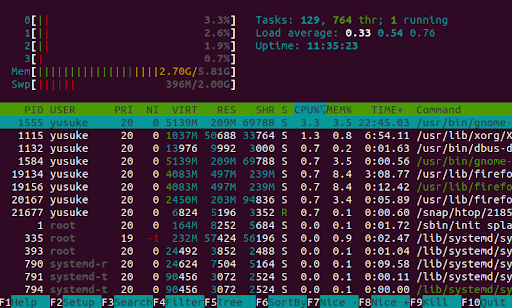
- The command
timechecks the overall performance of the code- By running this command, you get real time, user time and system time.
- Real is wall clock time - time from start to finish of the call. This includes the time of overhead
- User is the amount of CPU time spent outside the kernel within the process
- Sys is the amount of CPU time spent in the kernel within the process.
- User time +Sys time will tell you how much actual CPU time your process used.
Parallel Computing Challenges
Pre-Tasks
Make sure to clone a copy of your challenges repo onto M3, ideally in a personal folder on vf38_scratch.
Note: For every challenge you will be running the programs as SLURM jobs. This is so we don't overload the login nodes. A template SLURM job script is provided at the root of this directory which you can use to submit your own jobs to SLURM by copying it to each challenges sub-directory and filling in the missing details. You may need more than one for some challenges. This template will put the would-be-printed output in a file named
slurm-<job-name>.out.
Task 1 - Single Cluster Job using OpenMP
Create a program in hello.c that prints 'Hello, world from thread:
Note:
- The output of a job is put in a slurm-
.out file by default. - The template slurm job scripts will output the results to a
slurm-<job-name>.outfile.
Task 2 - Parallel for Loop
In array-gen.c implement a program that generates an array containing the numbers 0..10'000 elements (inclusive) using a for loop. Measure the execution time using the time Linux command. Now reimplement the program to utilise OpenMP's parallel for loop macros, measuring the execution time again. Is there any performance improvement? Are the elements still in the correct order and if not how can you fix this. Try experimenting with different sized arrays and element types. Again, extend the program to use multi-nodes.
Hint: You will likely need to allocate memory from the heap.
Task 3 - Parallel Reductions
In the C chapter we created a sum program that summed the elements of an array together. Using this as a base, create a new program that again computes the sum of the elements of an array but using OpenMP, comparing the execution time between the sequential and parallel versions. Is there any performance improvement? How would using a different binary operator change our ability to parallelize the the reduction?
If you have time, implement the sum but at each iteration, raise the current value to the power of the current accumulation divide by 100, adding this to the accumulation. Test a serial and parallel version. Is the parallel any faster?
Note:
module load gccto use newer version of gcc if you have error with something like-std=c99.
Task 4 - Laplace Equation for Calculating the Temperature of a Square Plane
For this challenge you will attempt to parallelize an existing implementation of the Laplace Equation. Throughout the source files of this project there are various loops you can try and make faster by utilizing OpenMP macros. See if you can make a faster version in the laplace2d-parallel.c. To build these files make sure you're in that directory and use the command make. The executables will be in the same directory.
Task 5 - Calculate Pi using "Monte Carlo Algorithm"
For this challenge you will have to try and implement the Monte Carlo algorithm with no framework or template and using everything you've learnt so far. Good luck.
Short explanation of Monte Carlo algorithm
Apache Spark
Apache Spark is an open-source, distributed computing system that has gained immense popularity for its speed, ease of use, and versatility in handling large-scale data processing tasks. Developed to overcome the limitations of the MapReduce paradigm, Spark offers a unified platform for various data processing workloads, including batch processing, real-time data streaming, machine learning, and graph processing.
Spark provides high-level APIs in languages like Scala, Java, Python, and R, making it accessible to a wide range of developers with different programming backgrounds.
In this chapter, we will:
- Set up a mini Spark cluster in M3.
- Take a closer look at the internal data structure, specifically Resilient Distributed Datasets (RDDs).
- Explore data processing in Spark and JupyterLab.
- Submit batch jobs utilizing both Slurm and Spark.
- Engage in some challenges.
Notes:
- The material covered in this chapter draws heavily from the official documentation of Spark 3.5.0.
- Contents of Setting up a Spark Cluster within M3 via Slurm and Submit Spark Job inside Slurm Job are both derived from a trial-and-error approach, and doesn't adhere to any official documentation. Consequently, there is a likelihood that it may not be the best practice. Thus, if you've discovered alternative methods or more effective approaches or may be even security vulnerabilities, please don't hesitate to submit a pull request.
Setting up a Spark cluster within M3 cluster
Installation
Different Spark version may have different version requirements for Python and Java. We will use Spark 3.5, Python 3.10 (JupyterLab Environment), and Java 8 (default in M3). There are 2 main things that we need to set up:
- Miniconda
Conda can be installed using the conda-install module from M3. The JupyterLab environment currently uses Python 3.10, meeting the prerequisite for Spark 3.5. This environment will also be utilized for running a notebook in STRUDEL. For those interested in customizing their own conda environment on M3, detailed instructions can be found in this page.
module load conda-install
conda-install
- Spark Engine
Since M3 does not include a built-in module for Spark, we need to download and unzip it. Other versions can be found here
# Spark 3.5.0
wget https://dlcdn.apache.org/spark/spark-3.5.0/spark-3.5.0-bin-hadoop3.tgz
tar xzfv spark-3.5.0-bin-hadoop3.tgz
rm -rf spark-3.5.0-bin-hadoop3.tgz
Getting the cluster running
Requesting nodes from M3
We can refer to the M3 chapter to request an interactive session. E.g:
# Interactive session with: 12 cpus, 1 hour of time, 4 nodes, 8gb memory per node on m3i partion
smux new-session --jobname=testing_spark --ntasks=4 --time=0-01:00:00 --partition=m3i --mem=8GB --nodes=4 --cpuspertask=4
Setting up worker
- Write requested nodes name to the config file within spark
# Get names of all nodes
# Read from 2nd node to the last node (as the 1st node is the master node)
# Write it to the config file workers within spark engine
scontrol show hostnames | sed -n '2,$p' > /path/to/spark-3.5.0-bin-hadoop3/conf/workers
Starting spark cluster
- Start the cluster
source /path/to/spark-3.5.0-bin-hadoop3/sbin/start-all.sh
Connecting Jupyter Lab (STRUDEL) to the Cluster
Spark’s shell offers a straightforward approach to grasp the API and serves as a robust tool for interactive data analysis. However, incorporating a user-friendly interface facilitates more intricate operations and functionalities. In this context, we'll utilise Jupyter Lab, which is made available through STRUDEL.
Requesting a notebook through STRUDEL
When installing miniconda in M3, there will be a built-in environment named jupyterlab. This environment will also be automatically added into STRUDEL and we can launch a JupyterLab session from this environment.
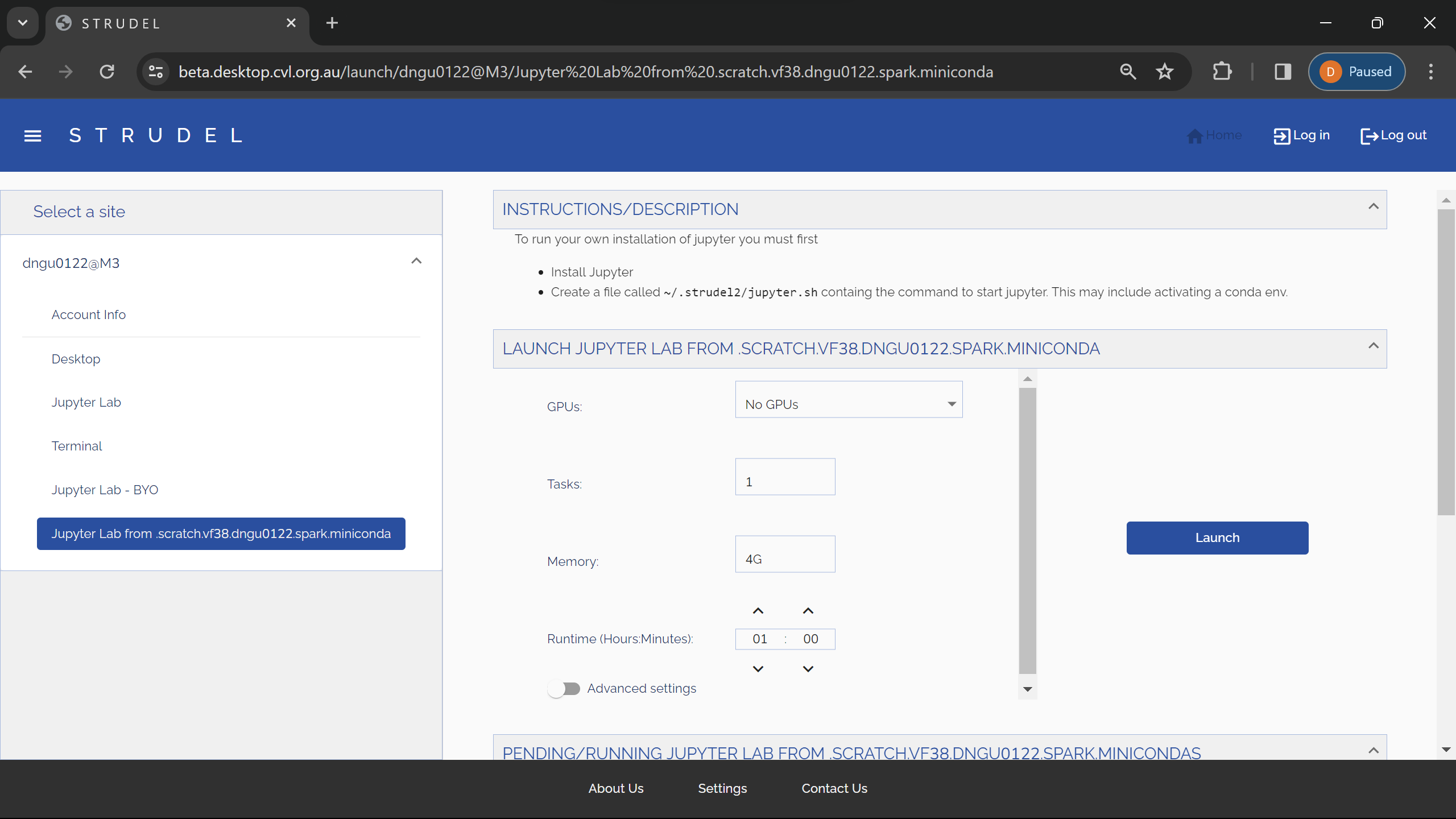
Exporting environments variables
import sys
import os

# Specify paths, which will be set as environment variables and read by the Spark engine
SPARK_HOME = "/path/to/spark-3.5.0-bin-hadoop3"
os.environ["SPARK_HOME"] = SPARK_HOME
PREV_PATH = os.environ["PATH"]
os.environ["PATH"] = f"{SPARK_HOME}/bin:{PREV_PATH}"

# Specify which Python to be used by the driver and workers
os.environ["PYSPARK_PYTHON"] = sys.executable

# Add pyspark to the PYTHONPATH
PYSPARK_HOME=f"{SPARK_HOME}/python"
sys.path.append(PYSPARK_HOME)

# Different Spark version will have different py4j version
sys.path.append(f"{PYSPARK_HOME}/lib/py4j-0.10.9.7-src.zip")
Connecting to the Spark master
import pyspark
from pyspark.sql import SparkSession

# Initilize a Spark context from the Spark Cluster
spark = SparkSession \
    .builder \
    .master("spark://{master_node}.massive.org.au:7077") \
    .appName("test") \
    .config("spark.workers.show", "True") \
    .getOrCreate()
SSH Tunnel SparkUI to Localhost
We can use ssh tunneling to forward the Spark UI of the engine to our local machine, the UI will be available as a web application at http://localhost:4040.
# The jupyterlab node will be the node that the jupyter lab is currently running on
ssh -L 4040:{jupyterlab_node}.massive.org.au:4040 {username}@m3.massive.org.au
Overview of what we have just done
The overall architecture can be demonstrated through this diagram:
- Each circle is a computing node of M3.
- A mini-cluster managed by Spark is running inside the big M3 cluster.
- We also have a notebook (from STRUDEL) connecting to the master node of the Spark cluster.
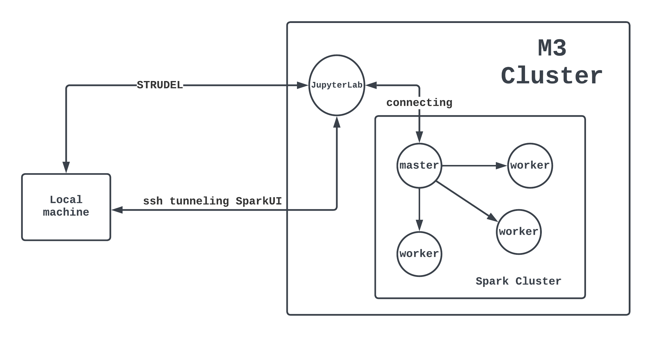
Spark Architecture Overview
Here is a diagram representing components of Apache Spark:
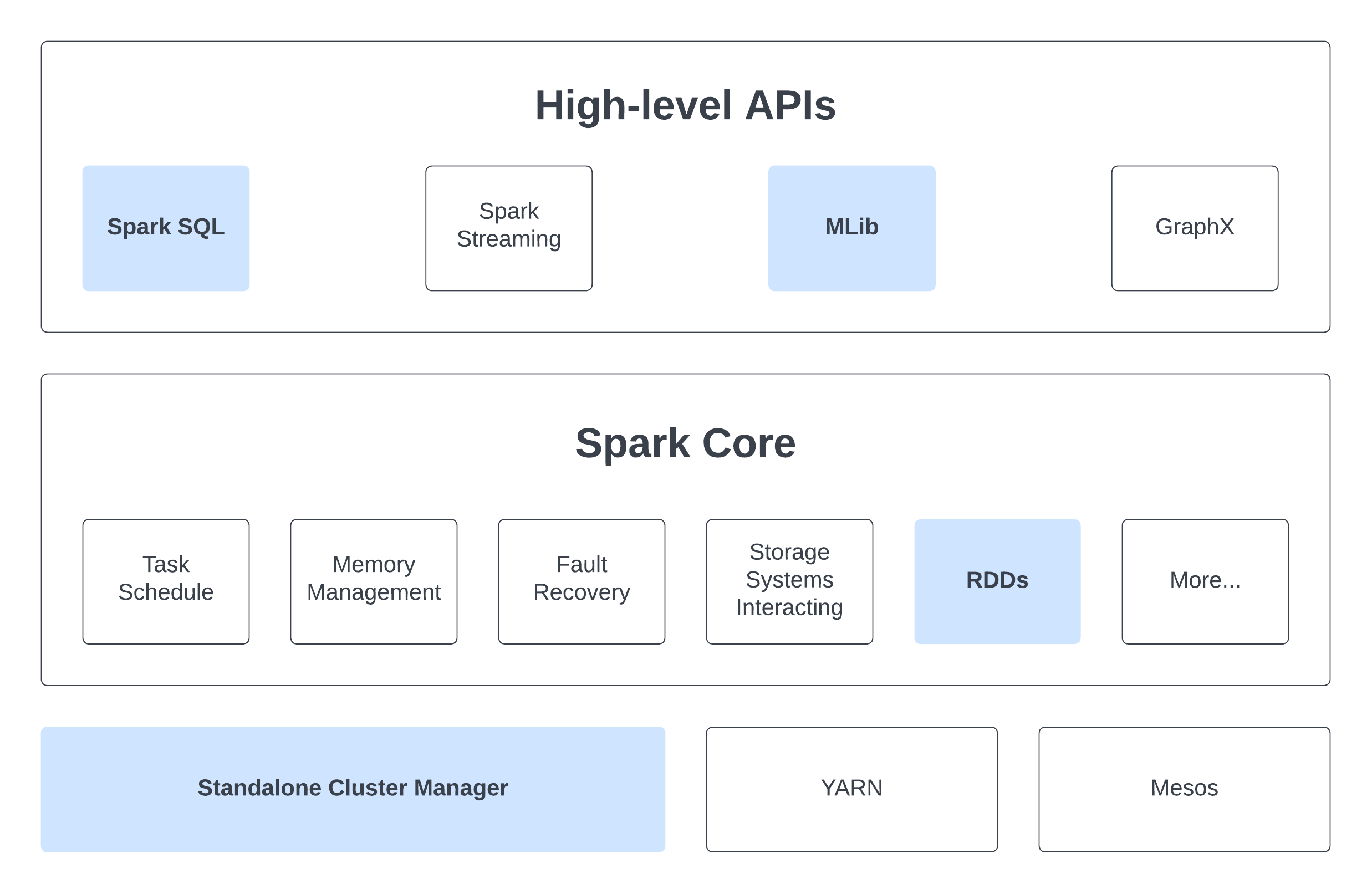
Within this chapter, we only look at components with blue boxes.
Cluster Managers
Spark is designed to smoothly scale from just one compute node to potentially thousands. It achieves this scalability while prioritizing flexibility by supporting various cluster managers, including Hadoop YARN, Apache Mesos, and its own Standalone Scheduler. For our setup, we've opted for the simplicity of the Standalone Scheduler to run a mini-cluster in the last section.
Spark Core - Resillient Distributed Datasets (RDDs)
What is RDDs?
RDD is simply an immutable distributed collection of objects. Within Spark, all tasks involve either generating new RDDs, modifying existing ones, or executing operations on RDDs to produce an outcome. Behind the scenes, Spark seamlessly disperses the data stored within RDDs into multiple partitions across your cluster and parallelizes the tasks you execute on them. Moreover, RDD can accommodate Python, Java, or Scala objects of any type, including user-defined classes. RDDs enable users to explicitly persist intermediate outcomes in memory, control their partitioning to optimize data distribution, and manipulate them using a diverse set of operators.
Initialize RDD
Parallelize Collections
We can create a RDD from an existing iterable or collection
data: list = ["H", "e", "l", "l", "o", "!"]

# by default, set the number of partitions automatically based on your cluster
chars: RDD = spark_context.parallelize(data)

# you can also set it manually by passing it as a second parameter to parallelize
chars: RDD = spark_context.parallelize(data, 10)
Read from External Datasets
PySpark can create distributed datasets from any storage source supported by Hadoop, including your local file system, HDFS, Cassandra, HBase, Amazon S3,...
# takes a URI for the file (either a local path on the machine, or a hdfs://, s3a://, etc URI)
# reads it as a collection of lines
lines: RDD = spark_context.textFile("/path/to/hello.txt")
Once created, RDD can be performed on by a diverse list of functional-style operations.
RDD Operations
Transformations and Actions
RDDs support two types of operations transformations and actions:
- Transformations are operations on RDDs that return a new RDD by applying the same operation to many data items. Transformations are
lazily evaluated(including loading data), it will only be computed when an action is called. Spark internally records metadata to indicate that a transformation has been requested. - Actions are operations that run computation on a RDD then return a value (non-RDD) or export data to a storage system.
Why laziness?
Many popular cluster computing frameworks (such as MapReduce and Dryad) offer high-level operators for parallel computations, simplifying work distribution and fault tolerance concerns. However, they lack abstractions for efficiently optimizing distributed memory when dealing with applications that frequently reuse intermediate results (iterative methods, interactive data mining, etc).
Within the majority of these frameworks, the exclusive method for reusing data between computations (e.g., between two MapReduce jobs) involves storing it in an external stable storage system, such as a distributed file system, resulting in significant overhead due to data replication, disk I/O operations, and serialization. Therefore, we will often have to spend time considering how to group together operations to minimize the number of MapReduce passes through our data.
Spark employs lazy evaluation to:
- Minimize the number of passes it makes over the data by consolidating operations.
- Allow more rich and flexible combinations of Transformations.
APIs Reference
A complete list of PySpark APIs is available at Apache Spark Documentation. If you're ever uncertain about whether a specific function is a transformation or an action, simply check its return type: transformations return RDDs, whereas actions return some other data type.
Examples
Let's look at a few simple examples of using PySpark
You should follow these examples on a JupyterLab connecting to a Spark Cluster
Monte Carlo Pi Estimation
import pyspark
from pyspark.sql import SparkSession
from random import random
from operator import add

# Set this to the name of the current master node of the Spark Cluster
# Eg: master_node = "m3i014"
master_node = ...

###### Initilize Spark Session ######
spark = SparkSession \
    .builder \
    .master(f"spark://{master_node}.massive.org.au:7077") \
    .appName("PythonJupyter") \
    .config("spark.workers.show", "True") \
    .getOrCreate()

###### Monte Carlo Pi Estimation ######

partitions = 4
n = 1000 * partitions
data = range(1, n + 1)

def point(_: int) -> float:
    x = random() * 2 - 1
    y = random() * 2 - 1
    return 1 if x ** 2 + y ** 2 <= 1 else 0

count = spark
    .sparkContext \
    # distribute data into partitions across cluster, we have the starting RDD here
    .parallelize(data, partitions) \
    # Transformation: map each data through a function, resulting in a new RDD
    .map(point) \
    # Action: Reduce all the data into a value
    .reduce(add)

print("Pi is roughly %f" % (4.0 * count / n))
Sort a Text File
# Randomly generate number and store in a file called "rand_ints.csv"
# Note: This is bash command
for i in {1..1000}; do echo $[($RANDOM)]; done > ./rand_ints.csv
from typing import Tuple
from pyspark.rdd import RDD
from pyspark.sql import SparkSession

# Set this to the Path of the file rand_ints.csv
# Note: Don't use Relative Path
file_path = ...
lines = spark \
    .read \
    .text(file_path) \
    .rdd \
    .map(lambda r: r[0])

sortedCount: RDD[Tuple[int, int]] = lines \
    .flatMap(lambda x: x.split(' ')) \
    .map(lambda x: (int(x), 1)) \
    .sortByKey()
Shared Variables
Typically, when a function is passed to a Spark operation like map or reduce and executed on a remote cluster node, it operates on separate copies of all the variables used within the function. These variables are duplicated across each machine, and any updates made to these variables on the remote machine are not communicated back to the driver program. Fortunately, Spark does provide 2 types of shared variables: Broadcast variables and Accumulators
Broadcast variables
Broadcast variables allow the program to efficiently send a large, read-only value to all the worker nodes for use in one or more Spark operations exactly once. The broadcasted variable will stay in each node until one of these cases:
- All tasks are finished.
- A
unpersist()method is called. However, this method will only release the resources in the executor node (the variable will be re-broadcasted again when it is used). - A
destroy()is called. This time, the variable can't be used again.
Note that these methods do not block by default! To block until resources are freed, specify
blocking=truewhen calling them.
broadcastVar = spark_context.broadcast([1, 2, 3])
print(broadcastVar.value) # [1, 2, 3]
Accumulators
Another type of shared variable, accumulators, provides a simple syntax for aggregating values from worker nodes back to the driver program.
Note that it is possible aggregate values from an entire RDD back to the driver program using actions (e.g:
reduce()). However, in the case when we want a simpler way to calculate a metric at some point in the program (e.g: count the number of the word "Hello" in a distributed text data), accumulator will be a handly solution.
accum = spark_context.accumulator(0)
spark_context.parallelize([1, 2, 3, 4]).foreach(lambda x: accum.add(x))
print(accum.value) # 10
Data Processing with Spark
Spark SQL
Spark SQL, a module of Spark, is designed for structured data processing. Unlike the basic Spark RDD API, the interfaces in Spark SQL offer more details about the data's structure and the ongoing computation. Internally, Spark SQL utilizes this additional information to make optimizations for improved performance.
Architecture Overview
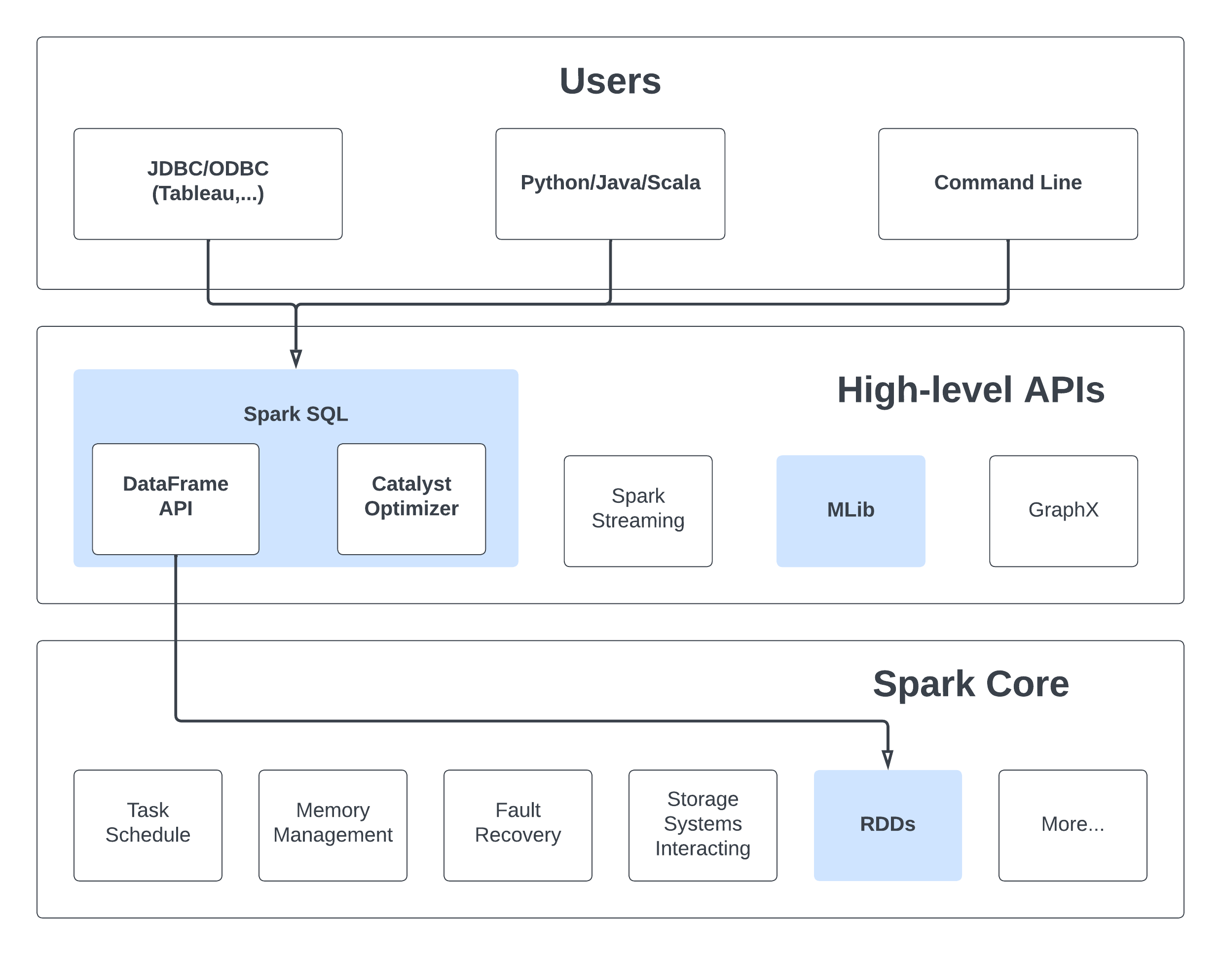
Capabilities
Spark SQL provides 3 main capabilities:
- Load data from a variety of structured sources (e.g., JSON, Hive, and Parquet).
- Query the data using SQL, both inside a Spark program and from external tools that connect to Spark SQL through standard database connectors (JDBC/ODBC), such as business intelligence tools like Tableau.
- Provides rich integration between SQL and regular Python/Java/Scala code, including the ability to join RDDs and SQL tables, expose custom functions in SQL, and more. Many jobs are easier to write using this combination.
Datasets and DataFrames
A Dataset represents a distributed assembly of data, combining the advantages of Resilient Distributed Datasets (RDDs) with the efficiency of Spark SQL's optimized execution engine.
Meanwhile, a DataFrame is a structured form of a Dataset, arranged into columns. It parallels the notion of a table in a relational database or a data frame in languages like R or Python, yet incorporates more sophisticated optimizations internally.
Working with PySpark DataFrames
We will now have a look at the examples provided in
path/to/spark-3.5.0-bin-hadoop3/examples/src/main/python/sql/basic.py
Job Batching
spark-submit
The spark-submit script found in Spark's bin directory serves to initiate applications on a cluster. It seamlessly integrates with all of Spark's supported cluster managers via a unified interface, eliminating the need for specific configuration adjustments tailored to each one individually.
# Remember to change the master_node to actual master node's name
source /path/to/spark-3.5.0-bin-hadoop3/bin/spark-submit \
    --master spark:{master_node}:7077 \
    hello_world.py
Here is a comprehensive documentation of all
spark-submitoptions. We will not look into the detail of it (If you need to find any command, it should be better to look directly into the documentation itself).We will focus on M3 and see how we can bundle and submit everything as Slurm jobs.
Slurm and Spark
Here is a complete bash script that we can sbatch to M3. We will now go through what is happening here:
#!/bin/bash
#SBATCH --job-name=SparkSlurm
#SBATCH --nodes=4
#SBATCH --time=00:15:00
#SBATCH --ntasks=1
#SBATCH --mem-per-cpu=4096
#SBATCH --cpus-per-task=1
#SBATCH --partition=m3i

############################ Spark Cluster #######################################

# This is basically the same steps as seen in the first subchapter

# Remember to change this to the actual path
export SPARK_HOME="/path/to/spark-3.5.0-bin-hadoop3"

# Add to the global PATH
export PATH="${SPARK_HOME}/bin:${PATH}"

 # Get all worker nodes and write to the config file of Spark
scontrol show hostnames | sed -n '2,$p' > $SPARK_HOME/conf/workers

# Start the spark cluster
$SPARK_HOME/sbin/start-all.sh

################################### Submit Job ###################################

# Get the master node, which will be the first node from the command `scontrol show hostnames`
master_node=$(scontrol show hostnames | head -1)

# Submit job to the Spark Cluster using spark-submit
# In this script we submit a provided example in the spark directory
$SPARK_HOME/bin/spark-submit \
    --master spark://${master_node}:7077 \
    $SPARK_HOME/examples/src/main/python/pi.py \
    1000
Apache Spark Challenges
Overview
Note: Tasks 1, 2, and 3 closely resemble a typical workflow when working with Apache Spark:
- Step 1: Interactively work with a small sample of the problem
- Step 2: Solve and optimize the sample problem
- Step 3: Submit the entire larger problem as a batch job
- Step 4: Analyze the result and, if necessary, repeat steps 1 to 4
You should employ this workflow into task 4 and task 5
Task 1 - Classic Distributed Problem: Token Counting
Given a string of tokens, count the number of times each token apprears. You should do this task in an interactive JupyterLab notebook connecting to a Spark cluster. This is a cananical problem of distributed data processing, and often served as an example for MapReduce Programming Model.
Hint: Have a look at map() and reduceByKey()
Task 2 - Cluster Set-up Bash Scripts
Write Bash Scripts to streamline the process of installing Spark and running the cluster.
Hint: Try to combine the subchapter: set up
Task 3 - Spark and Slurm
Submit task 1 as a Spark job using Slurm. This should be similar to subchapter: job batching
Hint:
- You will need to convert the notebook into a Python file.
- Compare the content of
$SPARK_HOME/examples/src/main/python/pi.pyand our Monte Carlo Pi Estimation. They both solve the same problem, however, there are stuffs that we don't need to add when directly usingspark-submit. Why?
Task 4 - Data Processing
In this task, we will start working witha dataframe and try to process a given real-world dataset.
The dataset, at around ~100MB, is considered small and not well-suited for Spark utilization (opting for Pandas might be more efficient). Nevertheless, working with this dataset serves as an exercise to understand more about Spark concepts and its capabilities.
Task 5 - Spark Machine Learning
We will use the data from task 4 to build an intro-to-Machine-Learning model, Linear Regression, with MLlib
Applying HPC
Now that you learnt what HPC is in the context of parallel & distributed computing, let's learn how you'd actually apply it to solve real-world problems.
CPU-bound vs. IO-bound
We can roughly divide up HPC application paradigms into two based on where the performance bottleneck is. If the computer program you're trying to speed up doesn't really need to work with large datasets but hogs the CPU a lot then we call them CPU-bound processes. On the other hand, if there's a ton of data extraction, transformation and loading with really large datasets then we call them IO-bound processes. It's useful to know this since how we write highly performant code depends on which of these categories the solution falls into.
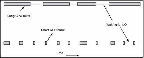
Considerations:
- For CPU-bound tasks, it's important to minimize the number of threads to avoid overloading the CPU, as well as to ensure that each thread has enough CPU time to complete its work. This may involve using techniques such as task prioritization or work stealing to balance the load between threads.
- For IO-bound tasks, it's important to use a large pool of threads to take advantage of the fact that these tasks spend a significant amount of time waiting for I/O operations to complete. This allows multiple IO-bound tasks to run concurrently on separate threads, maximizing the use of available I/O bandwidth and reducing the overall time taken to complete these tasks.
We will now delve into two of the most popular domains where HPC is needed - Machine Learning & Optimisation Algorithms. Machine learning as you might know, involves working with large amounts of data so therefore we will have to speed up IO-bound tasks. Whereas, optimisation typically involves more time on the CPU to compute a large amount of permutations of various solutions so the bottleneck here is CPU walltime instead.
Note: In this context, we're referring to non-regression based optimisation. So think more along the lines of root finding using heuristic algorithms rather than predicting the best solution based on statistical regression i.e. machine learning.
Machine Learning & HPC
What is Machine Learning?
Machine learning is a subset of artificial intelligence that involves developing AI models that enable computers to learn from and make predictions or decisions based on vast amounts of data. It pertains to training the model on these large datasets to identify patterns and insights, and automatically learn about these data to predict results from new, unseen data. The training datasets contain pre-determined outputs and their respective inputs, allowing the ML model to pick up patterns that enable these outputs to occur.
How a ML model is trained
During the training phase of a ML algorithm, it uses the training dataset to predict the output, and then compares the predicted output to the actual output to measure the disparity and compute the loss. Next, the gradient of the loss against the model parameters is calculated and used to update the model parameters via gradient descent. This process is repeated for a specific number of times or until the loss is below a certain threshold.

Since ML algorithms often deal with massive training datasets and complex models, the training usually takes a very long time and requires significant computational resources. HPC provides a way to speed this process up by distributing the dataset or model across different nodes/GPUs. There are two main forms of parallelism - Data Parallelism and Model Parallelism.
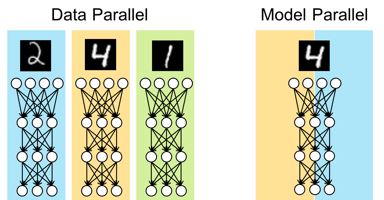
Data Parallelism
Data parallelism involves dividing and distributing the training dataset across multiple nodes/GPUs. Each node receives a copy of the ML model, and they individually process their portion of the data to compute the gradient. The gradients are then averaged and the weights in all the models in all the nodes are appropriately tuned. Data parallelism is more suited for instances where the training dataset is massive and the individual samples can be processed independently, such as CNNs.
Model Parallelism
Model parallelism involves partitioning the layers of the model across nodes/GPUs, allowing different parts of the model to process different batches of data simultaneously. Each node receives a layer of the ML model, and these nodes are aligned in a way that the output of one node is an input to another. These nodes individually process a different batch of data simultaneously, and then pass the data and activations to the next node. The same batch of data is passed from one node to another, with the next batch following right after. Model parallelism is more suited for models with large memory requirements or complex architectures, such as NLPs.
Optimisation Algorithms
Optimisation algorithms are a family of algorithms which aim to find the best combination of some variables, to maximise (or minimise) some kind of output. Though that may sound quite abstract, optimisation algorithms can in fact be applied to a variety of different practical problems. Some examples where optimisation algorithms could be used include:
- An bakery trying to figure out which ingredients to buy to maximise profit
- A small business owner attempting to create the 'optimal' shift for their workers
- A deep learning engineer trying to find the best parameters for their artificial intelligence model
Though at surface level all these problems may look appear quite different, each of these situations can be modelled mathematically in similar ways, allowing us to use techniques from linear algebra to help us out.
Linear Algebra
One can think of optimisation algorithms as an attempt to answer the question "what is the best choice one can make right now?" In order to find the best choice, we should figure out some way to organise the choices we can make.
In virtually all cases, one can model the list of all choices as just a list of numbers, with each number corresponding to one parameter that can be adjusted, for example
- If the bakery has 10 ingredients, then the numbers could be an (ordered) list of the amount of each ingredient
- The small business owner can represent a whole shift as a list of numbers, each number corresponding the shifts of each worker
- The deep learning engineer probably has a list of parameters already, and they just need to fine tune the coefficients
This is very similar to the coordinate system taught in high school. The same way we think of two numbers in a coordinate system as a point on the plane (like (0,0) being at the centre of the xy plane), we can think of these lists of numbers as points on some higher dimensional plane. See how even in the small example of the bakery with 10 ingredients, we're already dealing with 10 dimensional space. With the small AI, one might use a model with 128 parameters. Meaning, the mathematic represents some kind of 128-dimensional space.
If you can't imagine 128 dimensions of space, that's fine. what's important is that the logic and systems that are true in 2 or 3 dimensions are also true in higher dimensions. The analogy of "points in space" will also be useful in a bit. In mathematics jargon, one could say an optimisation problem with n variables can be modelled as a vector space with n+1 dimensions. Why n+1? see below.
Cost Function
Once we have a way of describing all the choices we can make, we need a way of saying how good each choice is. In other words, we need to take each point in our space, and associate this with some metric of "goodness". The better that point is, the higher number it receives. Mathematically, one would conceptualise this as a function which takes in the parameters as input, and outputs something outside of those parameters. That's where the extra +1 variable comes from
This metric would arise naturally out of the problem we are trying to study. For the bakery example, it would be something like how much profit each choice can generate. In the AI example, it would probably be the performance of the model.
Why do we need these algorithms?
Here's an exercise:
Draw a square of radius 10 and fill in with a bunch of dots in random positions. Then, cut out 10 circles of radius 1. Now I ask you the question, how many dots can you cover at most?
This is a very strange question, and its not immediately obvious how one would approach this problem. if the points were laid out in front of us, a human could probably intuit the best placement of circle cut outs. But building an algorithm that can reliably cover a good amount of circles is quite difficult.
That's the point of these algorithms. To construct a way for computers to mimic the human intuition of a strange and complicated problem. We'll see some algorithms that can do that in a bit. But first, some more weird functions.
Strange Functions
Here's some images of the output of functions

These are the Beale Contour, Rastrigin Contour, and the Rosenbrock Contour respectively. Notice that it is not immediately obvious how a computer should determine the minima (or maxima) of these functions. Checking every single point becomes radically exhaustive extremely quickly. So we need HPC for this.
Acknowledgements
This book is part of Monash DeepNeurons collection of technical information and internal training resources. It is built and maintained internally by members of Monash DeepNeuron.